The NIMBLE project anticipates having some funding for a part-time programmer to implement statistical algorithms and make improvements in nimble’s core code. Examples may include building adaptive Gaussian quadrature in nimble’s programming system and expanding nimble’s hierarchical model system. Remote work is possible. This is not a formal job solicitation, but please send a CV/resume to nimble.stats@gmail.com if you are interested so we can have you on our list. Important skills will be experience with hierarchical statistical modeling algorithms, R programming, and nimble itself. Experience with C++ will be helpful but not required.
Author Archives: nimble-admin
A close look at some posted trials of nimble for accelerated failure time models
A bunch of folks have brought to our attention a manuscript by Beraha, Falco and Guglielmi (BFG) posted on arXiv giving some comparisons between JAGS, NIMBLE, and Stan. Naturally, we wanted to take a look. Each package performs best in some of their comparisons. There’s a lot going on, so here we’re just going to work through the last of their four examples, an accelerated failure time (AFT) model, because that’s the one where NIMBLE looks the worst in their results. The code from BFG is given on GitHub here
There may be some issues with their other three examples as well, and we might work through those in future blog post(s). NIMBLE provides a lot of flexibility for configuring MCMCs in different ways (with different samplers), which means a comparison using our default configuration is just a start. Performance differences can also arise from writing the same model in different ways. We see both kinds of issues coming up for the other examples. But the AFT example gives a lot to talk about, so we’re sticking to that one here.
It turns out that NIMBLE and JAGS were put at a huge disadvantage compared to Stan, and that BFG’s results from NIMBLE don’t look valid, and that there isn’t any exploration of NIMBLE’s configurability. If we make the model for NIMBLE and JAGS comparable to the model for Stan, NIMBLE does roughly 2-45 times better in various cases than what BFG reported. If we explore a simple block sampling option, NIMBLE gets a small additional boost in some cases. It’s hard to compare results exactly with what BFG report, and we are not out to re-run the full comparison including JAGS and Stan. A “back of the envelope” comparison suggests that NIMBLE is still less efficient than Stan for this example, but not nearly to the degree reported. We’re also not out to explore many sampling configurations to try for better performance in this particular example problem, but part of NIMBLE’s design is to make it easy to do so.
Before starting into the AFT models, it’s worth recognizing that software benchmarks and other kinds of performance comparisons are really hard to do well. It’s almost inevitable that, when done by developers of one package, that package gets a boost in results even if objectivity is the honest goal. That’s because package developers almost can’t help using their package effectively and likely don’t know how to use other packages as well as their own. In this case, it’s fair to point out that NIMBLE needs more care in providing valid initial values (which BFG’s code doesn’t do) and that NIMBLE’s default samplers don’t work well here, which is because this problem features heavy right tails of Weibull distributions with shape parameter < 1. For many users, that is not a typical problem. By choosing slice samplers (which JAGS often uses too) instead of NIMBLE’s default Metropolis-Hastings samplers, the mixing is much better. This issue is only relevant to the problem as BFG formulated it for JAGS and NIMBLE and goes away when we put it on par with the formulation BFG gave to Stan. In principle, comparisons by third parties, like BFG, might be more objective than those by package developers, but in this case the comparisons by BFG don’t use JAGS or NIMBLE effectively and include incorrect results from NIMBLE.
Below we try to reproduce their (invalid) results for NIMBLE and to run some within-NIMBLE comparisons of other methods. We’ll stick to their model scenarios and performance metrics. Those metrics are not the way we’ve done some published MCMC comparisons here, here and here, but using them will allow readers to interpret our results alongside theirs.
First we’ll give a brief summary of their model scenarios. Here goes.
Accelerated Failure Time (AFT) models
Here’s a lightning introduction to AFT models based on Weibull distributions. These are models for time-to-event data such as a “failure.” For shape 


 = \frac{a}{s}\left(\frac{t}{s}\right)^{a-1} e^{-\left(\frac{t}{s}\right)^a}")
One important thing about the Weibull is that its cumulative density can be written in closed form. It is:
 = 1-e^{\left(\frac{t}{s}\right)^a}")
The role of covariates is to accelerate or decelerate the time course towards failure, effectively stretching or shrinking the time scale for each item. Specifically, for covariate vector 


 = \theta f_W(\theta t | a, s)")

 = f_W(t | a, \frac{s}{\theta})")
In the code, there are two parameterizations in play. The first is ")
^{-\frac{1}{a}} e^{x' \beta}")
^{a})")
 e^{-a(x' \beta)}")
The reason for the ")
")

alpha in the code) and beta). There is no separate scale parameter. Rather, ")
Right-censored failure time data
When a failure time is directly observed, its likelihood contribution is ")
")
There are two ways to handle a right-censored observation in MCMC:
- Include the likelihood factor
- Include a latent state,
, for the failure time. Include the likelihood factor
and let MCMC sample
The first version is marginalized relative to the second version because
It’s easy to set up the marginalized version for JAGS or NIMBLE. This can be done using the “zeroes” trick in the BUGS language, which both packages use for writing models. In NIMBLE this can also be done by writing a user-defined distribution as a nimbleFunction, which can be compiled along with a model.
BFG’s scenarios
BFG included the following scenarios:
- Sample size,
, is 100 or 1000.
- Number of explanatory variables,
, is 4 or 16. These always include an intercept. Other covariates, and the true coefficient values, are simulated.
- Censoring times are drawn from another Weibull distribution. This is set up following previous works such that the expected proportion of censored values is 20%, 50% or 80%.
- Most of their comparisons use informative priors. Those are the ones we look at here. Again, we weren’t out to look at everything they did.
- They used
total iterations. Of these,
were discarded as burn-in (warmup). They used a thinning interval of 2, resulting in
saved samples.
Some issues to explore
Now that we’ve set up the background, we are ready to list some of the issues with BFG’s comparisons that are worth exploring. For the computational experiments below, we decided to limit our efforts to NIMBLE because we are not trying to re-do BFG’s full analysis. Here are the main issues.
- BFG gave Stan a much easier problem than they gave JAGS and NIMBLE. Stan was allowed to use direct calculation of right-censored probabilities. These are complementary (right-tail) cumulative probability density calculations. NIMBLE and JAGS were made to sample latent failure times for censored items, even though they can be set up to use the cumulative calculations as well. Below we give NIMBLE a more comparable problem to the one given by BFG to Stan.
- It looks like BFG must not have obtained valid results from NIMBLE because they did not set up valid initial values for latent failure times. NIMBLE can be more sensitive to initial values (“inits”) than JAGS. We think that’s partly because NIMBLE uses a lot of adaptive random-walk Metropolis-Hastings samplers in its default MCMC configuration. In any case, NIMBLE gives warnings at multiple steps if a user should give attention to initial values. We give warnings instead of errors because a user might have plans to add initial values at a later step, and because sometimes MCMC samplers can recover from bad initial values. In the AFT example, the model does not “know” that initial values for latent failure times must be greater than the censoring times. If they aren’t, the likelihood calculations will return a
-Inf(or possiblyNA), which causes trouble for the samplers. Inspection of the model after MCMC runs using BFG’s code shows that even after 10000 iterations, the model likelihood is-Inf, so the results are invalid. It’s fair to say this is an issue in how to use NIMBLE, but it’s confusing to include invalid results in a comparison. - Even with valid initial values in BFG’s model formulation, NIMBLE’s default samplers do not do well for this example. In this post, we explore slice samplers instead. The problem is that the Weibull distributions in these scenarios give long right tails, due to simulating with shape parameter < 1. This corresponds to failure rates that decrease with time, like when many failures occur early and then those that don’t fail can last a long, long time. MCMC sampling of long right tails is a known challenge. In trial runs, we saw that, to some extent, the issue can be diagnosed by monitoring the latent failure times and noticing that they don’t mix well. We also saw that sometimes regression parameters displayed mixing problems. BFG report that NIMBLE’s results have mean posterior values farther from the correct values than given by the other tools, which is a hint that something is more deeply wrong. Slice samplers work much better for this situation, and it is easy to tell NIMBLE to use slice samplers, which we did.
- BFG’s code uses matrix multiplication for
in Stan, but not in NIMBLE or JAGS, even though they also support matrix multiplication. Instead, BFG’s code for NIMBLE and JAGS has a scalar declaration for each element of the matrix multiplication operation, followed by the sums that form each element of the result. We modify the code to use matrix multiplication. While we don’t often see this make a huge difference in run-time performance (when we’ve looked at the issue in other examples), it could potentially matter, and it definitely speeds up NIMBLE’s model-building and compilation steps because there is less to keep track of. An intermediate option would be to use inner products (
inprod). - It’s worth noting that all of these examples are fairly fast and mix fairly well. Some might disagree, but these all generate reasonable effective sample sizes in seconds-to-minutes, not hours-to-days.
- There are some minor issues, and we don’t want to get nit-picky. One is that we don’t see BFG’s code being set up to be reproducible. For example, not only is there no
set.seedso that others can generate identical data sets, but it looks like each package was given different simulated data sets. It can happen that MCMC performance depends on the data set. While this might not be a huge issue, we prefer below to give each package the same, reproducible, data sets. Another issue is that looking at average effective sample size across parameters can be misleading because one wants all parameters mixed well, not some mixed really well and others mixed poorly. But in these examples the parameters compared are all regression-type coefficients that play similar roles in the model, and the averaging doesn’t look like a huge issue. Finally, BFG decline to report ESS/time, preferring instead to report ESS and time and let readers make sense of them. We see ESS/time as the primary metric of interest, the number of effectively independent samples generated per second, so we report it below. This gives a way to see how both mixing (ESS) and computation time contribute to MCMC performance.
Setting up the example
We use BFG’s code but modify it to organize it into functions and make it reproducible. The source files for this document includes code chunks to run and save results. We are not running JAGS or Stan because we are not trying to reproduce a full set of comparisons. Instead we are looking into NIMBLE’s performance for this example. Since the main issue is that BFG gave NIMBLE and JAGS harder models than they gave Stan, we fix this in a way that is not NIMBLE-specific and should also work for JAGS.
Here is a summary of what the code does:
- Set up the twelve cases with informative priors included in the first twelve rows of BFG’s table 5, which has their AFT results.
- For each of the twelve cases, run:
- the original method of BFG, which gives invalid results but is useful for trying to see how much later steps improve over what BFG reported;
- a method with valid initial values and slice sampling, but still in the harder model formulation given by BFG;
- a method with the model formulation matching what BFG gave to Stan, using marginal probabilities for censored times and also using matrix multiplication;
- a method with the model formulation matching what BFG gave to Stan and also with one simple experiment in block sampling. The block sampler used is a multivariate adaptive random-walk Metropolis-Hastings sampler for all the regression coefficients. It sometimes helps to let these try multiple propose-accept/reject steps because otherwise
tries each time the sampler ran.
Although the original method of BFG seems to give invalid results, we include it so we can try to roughly compare performance (shown below) against what they report. However one difficulty is that processing with -Inf and NaN values can be substantially slower than processing with actual numbers, and these issues might differ across systems.
Results here are run on a MacBook Pro (2019), with 2.4 GHz 8-Core Intel Core i9, and OS X version 11.6.
Results
Here are the results, in a table that roughly matches the format of BFG’s Table 5. “Perc” is the average fraction of observations that are right-censored.
As best as we can determine:
- “ESS/Ns” is their “
“. This is the mean effective sample size of the (4 or 16) beta coefficients per saved MCMC iteration. The number of saved iterations,
is 2500. We used
coda::effectiveSizeto estimate ESS. We did not see in their code what method they used. This is another reason we can’t be sure how to compare our results to theirs. - “Nit/t” is their “
“, total number of iterations (10000) per computation time, not counting compilation time.
- We calculate “ESS/t”, which is the product of the previous two numbers divided by four, (ESS/Ns)*(Nit/t)/4. This is the mean effective sample size from the saved samples per total sampling time (including burn-in). One might also consider modifying this for the burn-in portion. The factor 4 comes from
= 4. We do it this way to make it easier to compare to BFG’s Table 5. They decline to calculate a metric of ESS per time, which we view as a fundamental metric of MCMC performance. An MCMC can be efficient either by generating well-mixed samples at high computational cost or generating poorly-mixed samples at low computational cost, so both mixing and computational cost contribute to MCMC efficiency.
|
BFG (invalid)
|
BFG+inits+slice
|
Marginal
|
Marginal+blocks
|
|||||||||
|---|---|---|---|---|---|---|---|---|---|---|---|---|
| ESS/Ns | Nit/t | ESS/t | ESS/Ns | Nit/t | ESS/t | ESS/Ns | Nit/t | ESS/t | ESS/Ns | Nit/t | ESS/t | |
| Perc = 0.2 | ||||||||||||
| N=100, p = 4, perc = 0.2 | 0.27 | 6844.63 | 465.80 | 0.52 | 2325.58 | 300.65 | 0.39 | 9775.17 | 951.09 | 0.27 | 16233.77 | 1109.06 |
| N=1000, p = 4, perc = 0.2 | 0.30 | 1127.27 | 84.71 | 0.55 | 306.22 | 41.83 | 0.41 | 1527.88 | 157.65 | 0.28 | 2490.04 | 171.47 |
| N=100, p = 16, perc = 0.2 | 0.19 | 3423.49 | 161.60 | 0.36 | 949.49 | 84.94 | 0.27 | 3717.47 | 248.99 | 0.29 | 5621.14 | 408.77 |
| N=1000, p = 16, perc = 0.2 | 0.08 | 404.22 | 7.80 | 0.57 | 98.86 | 14.16 | 0.41 | 591.82 | 61.12 | 0.30 | 1100.47 | 83.33 |
| Perc = 0.5 | ||||||||||||
| N=100, p = 4, perc = 0.5 | 0.05 | 7262.16 | 98.39 | 0.08 | 2572.68 | 54.45 | 0.38 | 10214.50 | 960.31 | 0.26 | 15060.24 | 990.34 |
| N=1000, p = 4, perc = 0.5 | 0.10 | 1106.32 | 26.96 | 0.10 | 298.23 | 7.25 | 0.44 | 1987.28 | 219.92 | 0.26 | 3074.09 | 196.19 |
| N=100, p = 16, perc = 0.5 | 0.06 | 3411.80 | 52.07 | 0.21 | 940.56 | 49.94 | 0.23 | 3955.70 | 229.94 | 0.28 | 5854.80 | 415.89 |
| N=1000, p = 16, perc = 0.5 | 0.07 | 339.29 | 5.88 | 0.07 | 95.90 | 1.66 | 0.41 | 601.90 | 61.98 | 0.31 | 1074.58 | 83.07 |
| Perc = 0.8 | ||||||||||||
| N=100, p = 4, perc = 0.8 | 0.03 | 6761.33 | 51.99 | 0.02 | 2297.79 | 10.79 | 0.24 | 9842.52 | 602.28 | 0.20 | 15151.52 | 763.36 |
| N=1000, p = 4, perc = 0.8 | 0.02 | 1013.27 | 5.16 | 0.02 | 265.58 | 1.50 | 0.39 | 1831.50 | 180.50 | 0.25 | 2856.33 | 176.27 |
| N=100, p = 16, perc = 0.8 | 0.04 | 3412.97 | 33.45 | 0.03 | 876.96 | 6.74 | 0.17 | 3853.56 | 166.26 | 0.23 | 5820.72 | 329.18 |
| N=1000, p = 16, perc = 0.8 | 0.01 | 395.99 | 1.22 | 0.05 | 95.33 | 1.22 | 0.39 | 560.54 | 54.91 | 0.29 | 1016.57 | 72.55 |
The left-most set of results (“BFG (invalid)”) is comparable to the right-most (“NIMBLE”) column of BFG’s Table 5, in the same row order for their first 12 rows. The simulated data sets are different. For that reason and the stochasticity of Monte Carlo methods, we shouldn’t expect to see exactly matching values. And of course the computations were run on different systems, resulting in different times. Again, these results are invalid.
The next column (“BFG+inits+slice”) gives results when BFG’s model formulation for JAGS and NIMBLE is combined with valid initialization and slice sampling in NIMBLE. We can see that valid sampling generally gives lower ESS/time than the invalid results.
The next column shows results when the problem is set up as BFG gave it to Stan, and NIMBLE’s default samplers are used. If we assume the left-most results are similar to what BFG report, but with times from the system used here, then the boost in performance is the ratio of ESS/time between methods. For example, in the last row, the marginal method is 54.91/1.22 = 45.01 times more efficient that what BFG reported. We can make a similar kind of ratio between Stan and NIMBLE from BFG’s results, which gave Stan as about 380 times more efficient than NIMBLE (although rounding error for “1%” could be a substantial issue here). Putting these together, Stan might really be about 8.4 times more efficient than NIMBLE for this case, which is the hardest case considered.
The last column shows results of the single experiment with alternative (block) samplers that we tried. In many cases, it gives a modest additional boost. Often with more work one can find a better sampling strategy, which can be worth the trouble for extended work with a particular kind of model. In the last row of our results, this gives about another 72.55 / 54.91 = 1.32 boost in performance, lowering the ratio to Stan to about 6.4. Again, we decided to limit this post to within-NIMBLE comparisons, and the comparisons to Stan based on BFG’s results should be taken with a grain of salt because we didn’t re-run them.
In summary, it looks like BFG gave Stan a different and easier accelerated failure time problem than they gave NIMBLE and JAGS. When given the same problem as they gave Stan, NIMBLE’s default samplers perform around 2 to 45 times better than what BFG reported.
NIMBLE is hiring a programmer
The NIMBLE development team is hiring for a one-year programmer position. We are looking for someone with R and C++ experience. There is also a possibility of a part-time position. The deadline for full consideration is February 12. Application information is here: https://aprecruit.berkeley.edu/JPF02822.
Spread the word: NIMBLE is looking for a post-doc
We have an opening for a post-doctoral scholar to work on methods for and applications of hierarchical statistical models using the NIMBLE software (https://r-nimble.org) at the University of California, Berkeley. NIMBLE is an R package that combines a new implementation of a model language similar to BUGS/JAGS, a system for writing new algorithms and MCMC samplers, and a compiler that generates C++ for each model and set of algorithms. The successful candidate will work with Chris Paciorek, Perry de Valpine, and potentially other NIMBLE collaborators to pursue a research program with a combination of building and applying methods in NIMBLE. Specific methods and application areas will be determined based on interests of the successful candidate. Applicants should have a Ph.D. in Statistics or a related discipline. We are open to non-Ph.D. candidates who can make a compelling case that they have relevant experience. The position is funded for two years, with an expected start date between October 2018 and June 2019. Applicants should send a cover letter, including a statement of how their interests relate to NIMBLE, the names of three references, and a CV to nimble.stats@gmail.com, with “NIMBLE post-doc application” in the subject. Applications will be considered on a rolling basis starting 15 October, 2018.
Quick guide for converting from JAGS or BUGS to NIMBLE
Converting to NIMBLE from JAGS, OpenBUGS or WinBUGS
NIMBLE is a hierarchical modeling package that uses nearly the same modeling language as the popular MCMC packages WinBUGS, OpenBUGS and JAGS. NIMBLE makes the modeling language extensible — you can add distributions and functions — and also allows customization of MCMC or other algorithms that use models. Here is a quick summary of steps to convert existing code from WinBUGS, OpenBUGS or JAGS to NIMBLE. For more information, see examples on r-nimble.org or the NIMBLE User Manual.
Main steps for converting existing code
These steps assume you are familiar with running WinBUGS, OpenBUGS or JAGS through an R package such as R2WinBUGS, R2jags, rjags, or jagsUI.
- Wrap your model code in nimbleCode({}), directly in R.
- This replaces the step of writing or generating a separate file containing the model code.
- Alternatively, you can read standard JAGS- and BUGS-formatted code and data files using
readBUGSmodel. - Provide information about missing or empty indices
- Example: If x is a matrix, you must write at least x[,] to show it has two dimensions.
- If other declarations make the size of x clear, x[,] will work in some circumstances.
- If not, either provide index ranges (e.g. x[1:n, 1:m]) or use the dimensions argument to nimbleModel to provide the sizes in each dimension.
- Choose how you want to run MCMC.
- Use nimbleMCMC() as the just-do-it way to run an MCMC. This will take all steps to
set up and run an MCMC using NIMBLE’s default configuration. - To use NIMBLE’s full flexibility: build the model, configure and build the MCMC, and compile both the model and MCMC. Then run the MCMC via runMCMC or by calling the run function of the compiled MCMC. See the NIMBLE User Manual to learn more about what you can do.
See below for a list of some more nitty-gritty additional steps you may need to consider for some models.
Example: An animal abundance model
This example is adapted from Chapter 6, Section 6.4 of Applied Hierarchical Modeling in Ecology: Analysis of distribution, abundance and species richness in R and BUGS. Volume I: Prelude and Static Models by Marc Kéry and J. Andrew Royle (2015, Academic Press). The book’s web site provides code for its examples.
Original code
The original model code looks like this:
cat(file = "model2.txt","
model {
# Priors
for(k in 1:3){                # Loop over 3 levels of hab or time factors
   alpha0[k] ~ dunif(-10, 10) # Detection intercepts
   alpha1[k] ~ dunif(-10, 10) # Detection slopes
   beta0[k] ~ dunif(-10, 10)  # Abundance intercepts
   beta1[k] ~ dunif(-10, 10)  # Abundance slopes
}

# Likelihood
# Ecological model for true abundance
for (i in 1:M){
   N[i] ~ dpois(lambda[i])
   log(lambda[i]) <- beta0[hab[i]] + beta1[hab[i]] * vegHt[i]
   # Some intermediate derived quantities
   critical[i] <- step(2-N[i])# yields 1 whenever N is 2 or less
   z[i] <- step(N[i]-0.5)     # Indicator for occupied site
   # Observation model for replicated counts
   for (j in 1:J){
      C[i,j] ~ dbin(p[i,j], N[i])
      logit(p[i,j]) <- alpha0[j] + alpha1[j] * wind[i,j]
   }
}

# Derived quantities
Nocc <- sum(z[])         # Number of occupied sites among sample of M
Ntotal <- sum(N[])       # Total population size at M sites combined
Nhab[1] <- sum(N[1:33])  # Total abundance for sites in hab A
Nhab[2] <- sum(N[34:66]) # Total abundance for sites in hab B
Nhab[3] <- sum(N[67:100])# Total abundance for sites in hab C
for(k in 1:100){         # Predictions of lambda and p ...
   for(level in 1:3){    #    ... for each level of hab and time factors
      lam.pred[k, level] <- exp(beta0[level] + beta1[level] * XvegHt[k])
      logit(p.pred[k, level]) <- alpha0[level] + alpha1[level] * Xwind[k]
   }
}
N.critical <- sum(critical[]) # Number of populations with critical size
}")
Brief summary of the model
This is known as an "N-mixture" model in ecology. The details aren't really important for illustrating the mechanics of converting this model to NIMBLE, but here is a brief summary anyway. The latent abundances N[i] at sites i = 1...M are assumed to follow a Poisson. The j-th count at the i-th site, C[i, j], is assumed to follow a binomial with detection probability p[i, j]. The abundance at each site depends on a habitat-specific intercept and coefficient for vegetation height, with a log link. The detection probability for each sampling occasion depends on a date-specific intercept and coefficient for wind speed. Kéry and Royle concocted this as a simulated example to illustrate the hierarchical modeling approaches for estimating abundance from count data on repeated visits to multiple sites.
NIMBLE version of the model code
Here is the model converted for use in NIMBLE. In this case, the only changes to the code are to insert some missing index ranges (see comments).
library(nimble)
Section6p4_code <- nimbleCode( {
    # Priors
    for(k in 1:3) {                # Loop over 3 levels of hab or time factors
      alpha0[k] ~ dunif(-10, 10) # Detection intercepts
      alpha1[k] ~ dunif(-10, 10) # Detection slopes
      beta0[k] ~ dunif(-10, 10)  # Abundance intercepts
      beta1[k] ~ dunif(-10, 10)  # Abundance slopes
    }

    # Likelihood
    # Ecological model for true abundance
    for (i in 1:M){
      N[i] ~ dpois(lambda[i])
      log(lambda[i]) <- beta0[hab[i]] + beta1[hab[i]] * vegHt[i]
      # Some intermediate derived quantities
      critical[i] <- step(2-N[i])# yields 1 whenever N is 2 or less
      z[i] <- step(N[i]-0.5)     # Indicator for occupied site
      # Observation model for replicated counts
      for (j in 1:J){
        C[i,j] ~ dbin(p[i,j], N[i])
        logit(p[i,j]) <- alpha0[j] + alpha1[j] * wind[i,j]
        }
    }

    # Derived quantities; unnececssary when running for inference purpose
    # NIMBLE: We have filled in indices in the next two lines.
    Nocc <- sum(z[1:100])         # Number of occupied sites among sample of M
    Ntotal <- sum(N[1:100])       # Total population size at M sites combined
    Nhab[1] <- sum(N[1:33])  # Total abundance for sites in hab A
    Nhab[2] <- sum(N[34:66]) # Total abundance for sites in hab B
    Nhab[3] <- sum(N[67:100])# Total abundance for sites in hab C
    for(k in 1:100){         # Predictions of lambda and p ...
      for(level in 1:3){    #    ... for each level of hab and time factors
        lam.pred[k, level] <- exp(beta0[level] + beta1[level] * XvegHt[k])
        logit(p.pred[k, level]) <- alpha0[level] + alpha1[level] * Xwind[k]
        }
      }
    # NIMBLE: We have filled in indices in the next line.
    N.critical <- sum(critical[1:100]) # Number of populations with critical size
  })
Simulated data
To carry this example further, we need some simulated data. Kéry and Royle provide separate code to do this. With NIMBLE we could use the model itself to simulate data rather than writing separate simulation code. But for our goals here, we simply copy Kéry and Royle's simulation code, and we compact it somewhat:
# Code from Kery and Royle (2015)
# Choose sample sizes and prepare obs. data array y
set.seed(1)                   # So we all get same data set
M <- 100                      # Number of sites
J <- 3                        # Number of repeated abundance measurements
C <- matrix(NA, nrow = M, ncol = J) # to contain the observed data

# Create a covariate called vegHt
vegHt <- sort(runif(M, -1, 1)) # sort for graphical convenience

# Choose parameter values for abundance model and compute lambda
beta0 <- 0                    # Log-scale intercept
beta1 <- 2                    # Log-scale slope for vegHt
lambda <- exp(beta0 + beta1 * vegHt) # Expected abundance

# Draw local abundance
N <- rpois(M, lambda)

# Create a covariate called wind
wind <- array(runif(M * J, -1, 1), dim = c(M, J))

# Choose parameter values for measurement error model and compute detectability
alpha0 <- -2                        # Logit-scale intercept
alpha1 <- -3                        # Logit-scale slope for wind
p <- plogis(alpha0 + alpha1 * wind) # Detection probability

# Take J = 3 abundance measurements at each site
for(j in 1:J) {
  C[,j] <- rbinom(M, N, p[,j])
}

# Create factors
time <- matrix(rep(as.character(1:J), M), ncol = J, byrow = TRUE)
hab <- c(rep("A", 33), rep("B", 33), rep("C", 34))  # assumes M = 100

# Bundle data
# NIMBLE: For full flexibility, we could separate this list
#         into constants and data lists.  For simplicity we will keep
#         it as one list to be provided as the "constants" argument.
#         See comments about how we would split it if desired.
win.data <- list(
    ## NIMBLE: C is the actual data
    C = C,
    ## NIMBLE: Covariates can be data or constants
    ##         If they are data, you could modify them after the model is built
    wind = wind,
    vegHt = vegHt,
    XvegHt = seq(-1, 1,, 100), # Used only for derived quantities
    Xwind = seq(-1, 1,,100),   # Used only for derived quantities
    ## NIMBLE: The rest of these are constants, needed for model definition
    ## We can provide them in the same list and NIMBLE will figure it out.
    M = nrow(C),
    J = ncol(C),
    hab = as.numeric(factor(hab))
)
Initial values
Next we need to set up initial values and choose parameters to monitor in the MCMC output. To do so we will again directly use Kéry and Royle's code.
Nst <- apply(C, 1, max)+1   # Important to give good inits for latent N
inits <- function() list(N = Nst,
                         alpha0 = rnorm(3),
                         alpha1 = rnorm(3),
                         beta0 = rnorm(3),
                         beta1 = rnorm(3))

# Parameters monitored
# could also estimate N, bayesian counterpart to BUPs before: simply add "N" to the list
params <- c("alpha0", "alpha1", "beta0", "beta1", "Nocc", "Ntotal", "Nhab", "N.critical", "lam.pred", "p.pred")
Run MCMC with nimbleMCMC
Now we are ready to run an MCMC in nimble. We will run only one chain, using the same settings as Kéry and Royle.
samples <- nimbleMCMC(
    code = Section6p4_code,
    constants = win.data, ## provide the combined data & constants as constants
    inits = inits,
    monitors = params,
    niter = 22000,
    nburnin = 2000,
    thin = 10)
## Detected C as data within 'constants'.
## |-------------|-------------|-------------|-------------|
## |-------------------------------------------------------|
Work with the samples
Finally we want to look at our samples. NIMBLE returns samples as a simple matrix with named columns. There are numerous packages for processing MCMC output. If you want to use the coda package, you can convert a matrix to a coda mcmc object like this:
library(coda)
coda.samples <- as.mcmc(samples)
Alternatively, if you call nimbleMCMC with the argument samplesAsCodaMCMC = TRUE, the samples will be returned as a coda object.
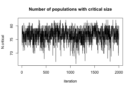
To show that MCMC really happened, here is a plot of N.critical:
plot(jitter(samples[, "N.critical"]), xlab = "iteration", ylab = "N.critical",
     main = "Number of populations with critical size",
     type = "l")
Next steps
NIMBLE allows users to customize MCMC and other algorithms in many ways. See the NIMBLE User Manual and web site for more ideas.
Smaller steps you may need for converting existing code
If the main steps above aren't sufficient, consider these additional steps when converting from JAGS, WinBUGS or OpenBUGS to NIMBLE.
- Convert any use of truncation syntax
- e.g. x ~ dnorm(0, tau) T(a, b) should be re-written as x ~ T(dnorm(0, tau), a, b).
- If reading model code from a file using readBUGSmodel, the x ~ dnorm(0, tau) T(a, b) syntax will work.
- Possibly split the data into data and constants for NIMBLE.
- NIMBLE has a more general concept of data, so NIMBLE makes a distinction between data and constants.
- Constants are necessary to define the model, such as nsite in for(i in 1:nsite) {...} and constant vectors of factor indices (e.g. block in mu[block[i]]).
- Data are observed values of some variables.
- Alternatively, one can provide a list of both constants and data for the constants argument to nimbleModel, and NIMBLE will try to determine which is which. Usually this will work, but when in doubt, try separating them.
- Possibly update initial values (inits).
- In some cases, NIMBLE likes to have more complete inits than the other packages.
- In a model with stochastic indices, those indices should have inits values.
- When using nimbleMCMC or runMCMC, inits can be a function, as in R packages for calling WinBUGS, OpenBUGS or JAGS. Alternatively, it can be a list.
- When you build a model with nimbleModel for more control than nimbleMCMC, you can provide inits as a list. This sets defaults that can be over-ridden with the inits argument to runMCMC.
NIMBLE workshop in Switzerland, 23-25 April
There will be a three-day NIMBLE workshop in Sempach, Switzerland, 23-25 April, hosted at the Swiss Ornithological Institute. More information can be found here: http://www.phidot.org/forum/viewtopic.php?f=8&t=3586. Examples will be oriented towards ecological applications, but otherwise the workshop content will be general.
Writing reversible jump MCMC in NIMBLE
Writing reversible jump MCMC samplers in NIMBLE
Introduction
Reversible jump Markov chain Monte Carlo (RJMCMC) is a powerful method for drawing posterior samples over multiple models by jumping between models as part of the sampling. For a simple example that I’ll use below, think about a regression model where we don’t know which explanatory variables to include, so we want to do variable selection. There may be a huge number of possible combinations of variables, so it would be nice to explore the combinations as part of one MCMC run rather than running many different MCMCs on some chosen combinations of variables. To do it in one MCMC, one sets up a model that includes all possible variables and coefficients. Then “removing” a variable from the model is equivalent to setting its coefficient to zero, and “adding” it back into the model requires a valid move to a non-zero coefficient. Reversible jump MCMC methods provide a way to do that.
Reversible jump is different enough from other MCMC situations that packages like WinBUGS, OpenBUGS, JAGS, and Stan don’t do it. An alternative way to set up the problem, which does not involve the technicality of changing model dimension, is to use indicator variables. An indicator variable is either zero or one and is multiplied by another parameter. Thus when the indicator is 0, the parameter that is multipled by 0 is effectively removed from the model. Darren Wilkinson has a nice old blog post on using indicator variables for Bayesian variable selection in BUGS code. The problem with using indicator variables is that they can create a lot of extra MCMC work and the samplers operating on them may not be well designed for their situation.
NIMBLE lets one program model-generic algorithms to use with models written in the BUGS language. The MCMC system works by first making a configuration in R, which can be modified by a user or a program, and then building and compiling the MCMC. The nimbleFunction programming system makes it easy to write new kinds of samplers.
The aim of this blog post is to illustrate how one can write reversible jump MCMC in NIMBLE. A variant of this may be incorporated into a later version of NIMBLE.
Example model
For illustration, I’ll use an extremely simple model: linear regression with two candidate explanatory variables. I’ll assume the first, x1, should definitely be included. But the analyst is not sure about the second, x2, and wants to use reversible jump to include it or exclude it from the model. I won’t deal with the issue of choosing the prior probability that it should be in the model. Instead I’ll just pick a simple choice and stay focused on the reversible jump aspect of the example. The methods below could be applied en masse to large models.
Here I’ll simulate data to use:
N <- 20
x1 <- runif(N, -1, 1)
x2 <- runif(N, -1, 1)
Y <- rnorm(N, 1.5 + 0.5 * x1, sd = 1)
I’ll take two approaches to implementing RJ sampling. In the first, I’ll use a traditional indicator variable and write the RJMCMC sampler to use it. In the second, I’ll write the RJMCMC sampler to incorporate the prior probability of inclusion for the coefficient it is sampling, so the indicator variable won’t be needed in the model.
First we’ll need nimble:
library(nimble)
RJMCMC implementation 1, with indicator variable included
Here is BUGS code for the first method, with an indicator variable written into the model, and the creation of a NIMBLE model object from it. Note that although RJMCMC technically jumps between models of different dimensions, we still start by creating the largest model so that changes of dimension can occur by setting some parameters to zero (or, in the second method, possibly another fixed value).
simpleCode1 <- nimbleCode({
    beta0 ~ dnorm(0, sd = 100)
    beta1 ~ dnorm(0, sd = 100)
    beta2 ~ dnorm(0, sd = 100)
    sigma ~ dunif(0, 100)
    z2 ~ dbern(0.8)  ## indicator variable for including beta2
    beta2z2 <- beta2 * z2
    for(i in 1:N) {
        Ypred[i] <- beta0 + beta1 * x1[i] + beta2z2 * x2[i]
        Y[i] ~ dnorm(Ypred[i], sd = sigma)
    }
})

simpleModel1 <- nimbleModel(simpleCode1,
                            data = list(Y = Y, x1 = x1, x2 = x2),
                            constants = list(N = N),
                            inits = list(beta0 = 0, beta1 = 0, beta2 = 0, sigma = sd(Y), z2 = 1))
Now here are two custom samplers. The first one will sample beta2 only if the indicator variable z2 is 1 (meaning that beta2 is included in the model). It does this by containing a regular random walk sampler but only calling it when the indicator is 1 (we could perhaps set it up to contain any sampler to be used when z2 is 1, but for now it’s a random walk sampler). The second sampler makes reversible jump proposals to move beta2 in and out of the model. When it is out of the model, both beta2 and z2 are set to zero. Since beta2 will be zero every time z2 is zero, we don’t really need beta2z2, but it ensures correct behavior in other cases, like if someone runs default samplers on the model and expects the indicator variable to do its job correctly. For use in reversible jump, z2’s role is really to trigger the prior probability (set to 0.8 in this example) of being in the model.
Don’t worry about the warning message emitted by NIMBLE. They are there because when a nimbleFunction is defined it tries to make sure the user knows anything else that needs to be defined.
RW_sampler_nonzero_indicator <- nimbleFunction(
    contains = sampler_BASE,
    setup = function(model, mvSaved, target, control) {
        regular_RW_sampler <- sampler_RW(model, mvSaved, target = target, control = control$RWcontrol)
        indicatorNode <- control$indicator
    },
    run = function() {
        if(model[[indicatorNode]] == 1) regular_RW_sampler$run()
    },
    methods = list(
        reset = function() {regular_RW_sampler$reset()}
    ))
## Warning in nf_checkDSLcode(code): For this nimbleFunction to compile, these
## functions must be defined as nimbleFunctions or nimbleFunction methods:
## reset.
RJindicatorSampler <- nimbleFunction(
    contains = sampler_BASE,
    setup = function( model, mvSaved, target, control ) {
        ## target should be the name of the indicator node, 'z2' above
        ## control should have an element called coef for the name of the corresponding coefficient, 'beta2' above.
        coefNode <- control$coef
        scale <- control$scale
        calcNodes <- model$getDependencies(c(coefNode, target))
    },
    run = function( ) { ## The reversible-jump updates happen here.
        currentIndicator <- model[[target]]
        currentLogProb <- model$getLogProb(calcNodes)
        if(currentIndicator == 1) {
            ## propose removing it
            currentCoef <- model[[coefNode]]
            logProbReverseProposal <- dnorm(0, currentCoef, sd = scale, log = TRUE)
            model[[target]] <<- 0
            model[[coefNode]] <<- 0
            proposalLogProb <- model$calculate(calcNodes)
            log_accept_prob <- proposalLogProb - currentLogProb + logProbReverseProposal
        } else {
            ## propose adding it
            proposalCoef <- rnorm(1, 0, sd = scale)
            model[[target]] <<- 1
            model[[coefNode]] <<- proposalCoef
            logProbForwardProposal <- dnorm(0, proposalCoef, sd = scale, log = TRUE)
            proposalLogProb <- model$calculate(calcNodes)
            log_accept_prob <- proposalLogProb - currentLogProb - logProbForwardProposal
        }
        accept <- decide(log_accept_prob)
        if(accept) {
            copy(from = model, to = mvSaved, row = 1, nodes = calcNodes, logProb = TRUE)
        } else {
            copy(from = mvSaved, to = model, row = 1, nodes = calcNodes, logProb = TRUE)
        }
    },
    methods = list(reset = function() {
    })
    )
Now we’ll set up and run the samplers:
mcmcConf1 <- configureMCMC(simpleModel1)
mcmcConf1$removeSamplers('z2')
mcmcConf1$addSampler(target = 'z2',
                     type = RJindicatorSampler,
                     control = list(scale = 1, coef = 'beta2'))
mcmcConf1$removeSamplers('beta2')
mcmcConf1$addSampler(target = 'beta2',
                     type = 'RW_sampler_nonzero_indicator',
                     control = list(indicator = 'z2',
                                    RWcontrol = list(adaptive = TRUE,
                                                   adaptInterval = 100,
                                                   scale = 1,
                                                   log = FALSE,
                                                   reflective = FALSE)))

mcmc1 <- buildMCMC(mcmcConf1)
compiled1 <- compileNimble(simpleModel1, mcmc1)
compiled1$mcmc1$run(10000)
## |-------------|-------------|-------------|-------------|
## |-------------------------------------------------------|
## NULL
samples1 <- as.matrix(compiled1$mcmc1$mvSamples)
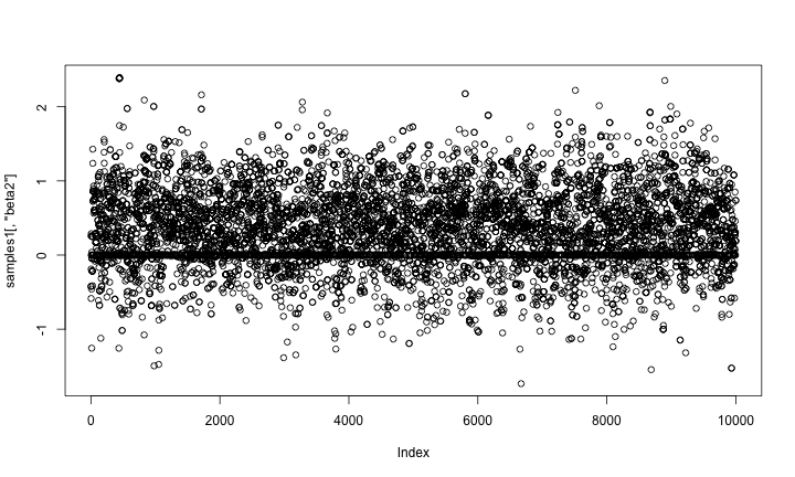
Here is a trace plot of the beta2 (slope) samples. The thick line at zero corresponds to having beta2 removed from the model.
plot(samples1[,'beta2'])
And here is a trace plot of the z2 (indicator variable) samples.
plot(samples1[,'z2'])
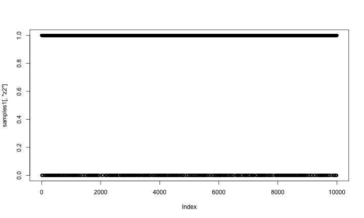
The chains look reasonable.
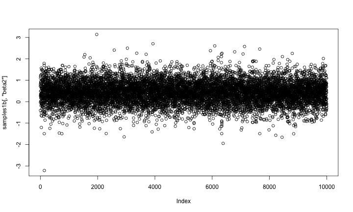
As a quick check of reasonableness, let’s compare the beta2 samples to what we’d get if it was always included in the model. I’ll do that by setting up default samplers and then removing the sampler for z2 (and z2 should be 1).
mcmcConf1b <- configureMCMC(simpleModel1)
mcmcConf1b$removeSamplers('z2')
mcmc1b <- buildMCMC(mcmcConf1b)
compiled1b <- compileNimble(simpleModel1, mcmc1b)
compiled1b$mcmc1b$run(10000)
## |-------------|-------------|-------------|-------------|
## |-------------------------------------------------------|
## NULL
samples1b <- as.matrix(compiled1b$mcmc1b$mvSamples)
plot(samples1b[,'beta2'])
qqplot(samples1[ samples1[,'z2'] == 1, 'beta2'], samples1b[,'beta2'])
abline(0,1)
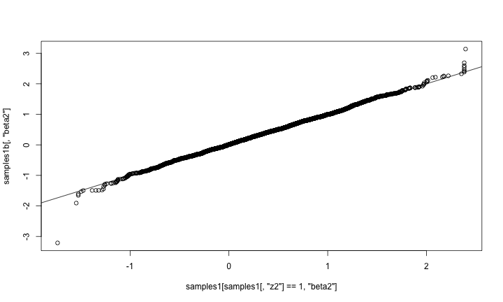
That looks correct, in the sense that the distribution of beta2 given that it’s in the model (using reversible jump) should match the distribution of beta2 when it is
always in the model.
RJ implementation 2, without indicator variables
Now I’ll set up the second version of the model and samplers. I won’t include the indicator variable in the model but will instead include the prior probability for inclusion in the sampler. One added bit of generality is that being “out of the model” will be defined as taking some fixedValue, to be provided, which will typically but not necessarily be zero. These functions are very similar to the ones above.
Here is the code to define and build a model without the indicator variable:
simpleCode2 <- nimbleCode({
    beta0 ~ dnorm(0, sd = 100)
    beta1 ~ dnorm(0, sd = 100)
    beta2 ~ dnorm(0, sd = 100)
    sigma ~ dunif(0, 100)
    for(i in 1:N) {
        Ypred[i] <- beta0 + beta1 * x1[i] + beta2 * x2[i]
        Y[i] ~ dnorm(Ypred[i], sd = sigma)
    }
})

simpleModel2 <- nimbleModel(simpleCode2,
                            data = list(Y = Y, x1 = x1, x2 = x2),
                            constants = list(N = N),
                            inits = list(beta0 = 0, beta1 = 0, beta2 = 0, sigma = sd(Y)))
And here are the samplers (again, ignore the warning):
RW_sampler_nonzero <- nimbleFunction(
    ## "nonzero" is a misnomer because it can check whether it sits at any fixedValue, not just 0
    contains = sampler_BASE,
    setup = function(model, mvSaved, target, control) {
        regular_RW_sampler <- sampler_RW(model, mvSaved, target = target, control = control$RWcontrol)
        fixedValue <- control$fixedValue
    },
    run = function() { ## Now there is no indicator variable, so check if the target node is exactly
                       ## equal to the fixedValue representing "not in the model".
        if(model[[target]] != fixedValue) regular_RW_sampler$run()
    },
    methods = list(
        reset = function() {regular_RW_sampler$reset()}
    ))
## Warning in nf_checkDSLcode(code): For this nimbleFunction to compile, these
## functions must be defined as nimbleFunctions or nimbleFunction methods:
## reset.
RJsampler <- nimbleFunction(
    contains = sampler_BASE,
    setup = function( model, mvSaved, target, control ) {
        ## target should be a coefficient to be set to a fixed value (usually zero) or not
        ## control should have an element called fixedValue (usually 0),
        ##    a scale for jumps to and from the fixedValue,
        ##    and a prior prob of taking its fixedValue
        fixedValue <- control$fixedValue
        scale <- control$scale
        ## The control list contains the prior probability of inclusion, and we can pre-calculate
        ## this log ratio because it's what we'll need later.
        logRatioProbFixedOverProbNotFixed <- log(control$prior) - log(1-control$prior)
        calcNodes <- model$getDependencies(target)
    },
    run = function( ) { ## The reversible-jump moves happen here
        currentValue <- model[[target]]
        currentLogProb <- model$getLogProb(calcNodes)
        if(currentValue != fixedValue) { ## There is no indicator variable, so check if current value matches fixedValue
            ## propose removing it (setting it to fixedValue)
            logProbReverseProposal <- dnorm(fixedValue, currentValue, sd = scale, log = TRUE)
            model[[target]] <<- fixedValue
            proposalLogProb <- model$calculate(calcNodes)
            log_accept_prob <- proposalLogProb - currentLogProb - logRatioProbFixedOverProbNotFixed + logProbReverseProposal
        } else {
            ## propose adding it
            proposalValue <- rnorm(1, fixedValue, sd = scale)
            model[[target]] <<- proposalValue
            logProbForwardProposal <- dnorm(fixedValue, proposalValue, sd = scale, log = TRUE)
            proposalLogProb <- model$calculate(calcNodes)
            log_accept_prob <- proposalLogProb - currentLogProb + logRatioProbFixedOverProbNotFixed - logProbForwardProposal
        }
        accept <- decide(log_accept_prob)
        if(accept) {
            copy(from = model, to = mvSaved, row = 1, nodes = calcNodes, logProb = TRUE)
        } else {
            copy(from = mvSaved, to = model, row = 1, nodes = calcNodes, logProb = TRUE)
        }
    },
    methods = list(reset = function() {
    })
    )
Now let’s set up and use the samplers
mcmcConf2 <- configureMCMC(simpleModel2)
mcmcConf2$removeSamplers('beta2')

mcmcConf2$addSampler(target = 'beta2',
                     type = 'RJsampler',
                     control = list(fixedValue = 0, prior = 0.8, scale = 1))
mcmcConf2$addSampler(target = 'beta2',
                     type = 'RW_sampler_nonzero',
                     control = list(fixedValue = 0,
                                     RWcontrol = list(adaptive = TRUE,
                                     adaptInterval = 100,
                                     scale = 1,
                                     log = FALSE,
                                     reflective = FALSE)))

mcmc2 <- buildMCMC(mcmcConf2)
compiled2 <- compileNimble(simpleModel2, mcmc2)

compiled2$mcmc2$run(10000)
## |-------------|-------------|-------------|-------------|
## |-------------------------------------------------------|
## NULL
samples2 <- as.matrix(compiled2$mcmc2$mvSamples)
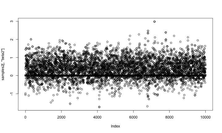
And again let’s look at the samples. As above, the horizontal line at 0 represents having beta2 removed from the model.
plot(samples2[,'beta2'])
Now let’s compare those results to results from the first method, above. They should match.
mean(samples1[,'beta2']==0)
## [1] 0.12
mean(samples2[,'beta2']==0)
## [1] 0.1173
qqplot(samples1[ samples1[,'beta2'] != 0,'beta2'], samples2[samples2[,'beta2'] != 0,'beta2'])
abline(0,1)
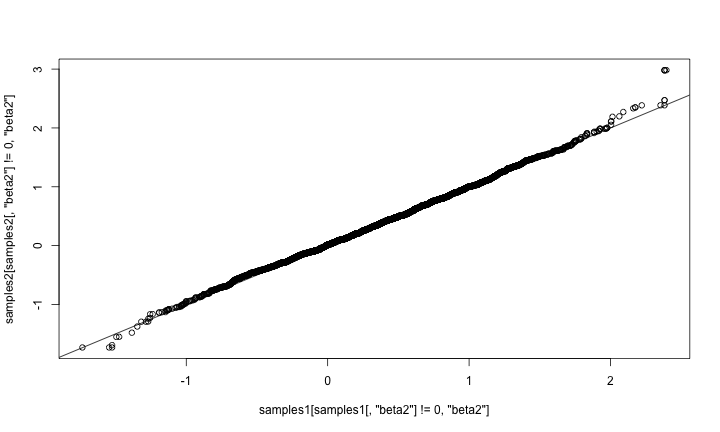
They match well. The samplers above could be assigned to arbitrary nodes in a model. The only additional code would arise from adding more samplers to an MCMC configuration. It would also be possible to refine the reversible-jump step to adapt the scale of its jumps in order to achieve better mixing. For example, one could try this method by Ehlers and Brooks. We’re interested in hearing from you if you plan to try using RJMCMC on your own models.
How to apply this for larger models.
En plus des crises existantes, le monde occidental a été frappé par une pénurie de médicaments. Et nous ne parlons pas principalement de la production de quelques molécules à forte intensité de main-d’œuvre, mais des médicaments fortlapersonne de base qui devraient se trouver dans chaque armoire à pharmacie, comme le paracétamol et les antibiotiques, dont la pénurie peut avoir un impact important sur la santé de la nation.
Building Particle Filters and Particle MCMC in NIMBLE
This example shows how to construct and conduct inference on a state space model using particle filtering algorithms. nimble currently has versions of the bootstrap filter, the auxiliary particle filter, the ensemble Kalman filter, and the Liu and West filter implemented. Additionally, particle MCMC samplers are available and can be specified for both univariate and multivariate parameters.
Model Creation
Assume 


")
")
with initial states
")
")
and prior distributions
")
")
where ")


")

We specify and build our state space model below, using 
## load the nimble library and set seed
library('nimble')
set.seed(1)

## define the model
stateSpaceCode <- nimbleCode({
    a ~ dunif(-0.9999, 0.9999)
    b ~ dnorm(0, sd = 1000)
    sigPN ~ dunif(1e-04, 1)
    sigOE ~ dunif(1e-04, 1)
    x[1] ~ dnorm(b/(1 - a), sd = sigPN/sqrt((1-a*a)))
    y[1] ~ dt(mu = x[1], sigma = sigOE, df = 5)
    for (i in 2:t) {
        x[i] ~ dnorm(a * x[i - 1] + b, sd = sigPN)
        y[i] ~ dt(mu = x[i], sigma = sigOE, df = 5)
    }
})

## define data, constants, and initial values
data <- list(
    y = c(0.213, 1.025, 0.314, 0.521, 0.895, 1.74, 0.078, 0.474, 0.656, 0.802)
)
constants <- list(
    t = 10
)
inits <- list(
    a = 0,
    b = .5,
    sigPN = .1,
    sigOE = .05
)

## build the model
stateSpaceModel <- nimbleModel(stateSpaceCode,
                              data = data,
                              constants = constants,
                              inits = inits,
                              check = FALSE)
Construct and run a bootstrap filter
We next construct a bootstrap filter to conduct inference on the latent states of our state space model. Note that the bootstrap filter, along with the auxiliary particle filter and the ensemble Kalman filter, treat the top-level parameters a, b, sigPN, and sigOE as fixed. Therefore, the bootstrap filter below will proceed as though a = 0, b = .5, sigPN = .1, and sigOE = .05, which are the initial values that were assigned to the top-level parameters.
The bootstrap filter takes as arguments the name of the model and the name of the latent state variable within the model. The filter can also take a control list that can be used to fine-tune the algorithm’s configuration.
## build bootstrap filter and compile model and filter
bootstrapFilter <- buildBootstrapFilter(stateSpaceModel, nodes = 'x')
compiledList <- compileNimble(stateSpaceModel, bootstrapFilter)
## run compiled filter with 10,000 particles.
## note that the bootstrap filter returns an estimate of the log-likelihood of the model.
compiledList$bootstrapFilter$run(10000)
## [1] -28.13009
Particle filtering algorithms in nimble store weighted samples of the filtering distribution of the latent states in the mvSamples modelValues object. Equally weighted samples are stored in the mvEWSamples object. By default, nimble only stores samples from the final time point.
## extract equally weighted posterior samples of x[10]  and create a histogram
posteriorSamples <- as.matrix(compiledList$bootstrapFilter$mvEWSamples)
hist(posteriorSamples)

The auxiliary particle filter and ensemble Kalman filter can be constructed and run in the same manner as the bootstrap filter.
Conduct inference on top-level parameters using particle MCMC
Particle MCMC can be used to conduct inference on the posterior distribution of both the latent states and any top-level parameters of interest in a state space model. The particle marginal Metropolis-Hastings sampler can be specified to jointly sample the a, b, sigPN, and sigOE top level parameters within nimble‘s MCMC framework as follows:
## create MCMC specification for the state space model
stateSpaceMCMCconf <- configureMCMC(stateSpaceModel, nodes = NULL)

## add a block pMCMC sampler for a, b, sigPN, and sigOE
stateSpaceMCMCconf$addSampler(target = c('a', 'b', 'sigPN', 'sigOE'),
                              type = 'RW_PF_block', control = list(latents = 'x'))

## build and compile pMCMC sampler
stateSpaceMCMC <- buildMCMC(stateSpaceMCMCconf)
compiledList <- compileNimble(stateSpaceModel, stateSpaceMCMC, resetFunctions = TRUE)
## run compiled sampler for 5000 iterations
compiledList$stateSpaceMCMC$run(5000)
## |-------------|-------------|-------------|-------------|
## |-------------------------------------------------------|
## NULL
## create trace plots for each parameter
library('coda')
par(mfrow = c(2,2))
posteriorSamps <- as.mcmc(as.matrix(compiledList$stateSpaceMCMC$mvSamples))
traceplot(posteriorSamps[,'a'], ylab = 'a')
traceplot(posteriorSamps[,'b'], ylab = 'b')
traceplot(posteriorSamps[,'sigPN'], ylab = 'sigPN')
traceplot(posteriorSamps[,'sigOE'], ylab = 'sigOE')

The above RW_PF_block sampler uses a multivariate normal proposal distribution to sample vectors of top-level parameters. To sample a scalar top-level parameter, use the RW_PF sampler instead.
NIMBLE package for hierarchical modeling (MCMC and more) faster and more flexible in version 0.6-1
NIMBLE version 0.6-1 has been released on CRAN and at r-nimble.org.
NIMBLE is a system that allows you to:
- Write general hierarchical statistical models in BUGS code and create a corresponding model object to use in R.
- Build Markov chain Monte Carlo (MCMC), particle filters, Monte Carlo Expectation Maximization (MCEM), or write generic algorithms that can be applied to any model.
- Compile models and algorithms via problem-specific generated C++ that NIMBLE interfaces to R for you.
Most people associate BUGS with MCMC, but NIMBLE is about much more than that. It implements and extends the BUGS language as a flexible system for model declaration and lets you do what you want with the resulting models. Some of the cool things you can do with NIMBLE include:
- Extend BUGS with functions and distributions you write in R as nimbleFunctions, which will be automatically turned into C++ and compiled into your model.
- Program with models written in BUGS code: get and set values of variables, control model calculations, simulate new values, use different data sets in the same model, and more.
- Write your own MCMC samplers as nimbleFunctions and use them in combination with NIMBLE’s samplers.
- Write functions that use MCMC as one step of a larger algorithm.
- Use standard particle filter methods or write your own.
- Combine particle filters with MCMC as Particle MCMC methods.
- Write other kinds of model-generic algorithms as nimbleFunctions.
- Compile a subset of R’s math syntax to C++ automatically, without writing any C++ yourself.
Some early versions of NIMBLE were not on CRAN because NIMBLE’s system for on-the-fly compilation via generating and compiling C++ from R required some extra work for CRAN packaging, but now it’s there. Compared to earlier versions, the new version is faster and more flexible in a lot of ways. Building and compiling models and algorithms could sometimes get bogged down for large models, so we streamlined those steps quite a lot. We’ve generally increased the efficiency of C++ generated by the NIMBLE compiler. We’ve added functionality to what can be compiled to C++ from nimbleFunctions. And we’ve added a bunch of better error-trapping and informative messages, although there is still a good way to go on that. Give us a holler on the nimble-users list if you run into questions.
NIMBLE: A new way to do MCMC (and more) from BUGS code in R
Yesterday we released version 0.5 of NIMBLE on our web site, r-nimble.org. (We’ll get it onto CRAN soon, but it has some special needs to work out.) NIMBLE tries to fill a gap in what R programmers and analysts can do with general hierarchical models. Packages like WinBUGS, OpenBUGS, JAGS and Stan provide a language for writing a model flexibly, and then they provide one flavor of MCMC. These have been workhorses of the Bayesian revolution, but they don’t provide much control over how the MCMC works (what samplers are used) or let one do anything else with the model (though Stan provides some additional fitting methods).
The idea of NIMBLE has been to provide a layer of programmability for algorithms that use models written in BUGS. We adopted BUGS as a model declaration language because these is so much BUGS code out there and so many books that use BUGS for teaching Bayesian statistics. Our implementation processes BUGS code in R and creates a model object that you can program with. For MCMC, we provide a default set of samplers, but these choices can be modified. It is easy to write your own sampler and add it to the MCMC. And it is easy to add new distributions and functions for use in BUGS code, something that hasn’t been possible (in any easy way) before. These features can allow big gains in MCMC efficiency.
MCMCs are heavily computational, so NIMBLE includes a compiler that generates C++ specific to a model and algorithm (MCMC samplers or otherwise), compiles it, loads it into R and gives you an interface to it. To be able to compile an algorithm, you need to write it as a nimbleFunction rather than a regular R function. nimbleFunctions can interact with model objects, and they can use a subset of R for math and flow-control. Among other things, the NIMBLE compiler automatically generates code for the Eigen C++ linear algebra library and manages all the necessary interfaces.
Actually, NIMBLE is not specific to MCMC or to Bayesian methods. You can write other algorithms to use whatever model you write in BUGS code. Here’s one simple example: in the past if you wanted to do a simulation study for a model written in BUGS code, you had to re-write the model in R just to simulate from it. With NIMBLE you can simulate from the model as written in BUGS and have complete control over what parts of the model you use. You can also query the model about how nodes are related so that you can make an algorithm adapt to what it finds in a model. We have a set of sequential Monte Carlo (particle filter) methods in development that we’ll release soon. But the idea is that NIMBLE provides a platform for others to develop and disseminate model-generic algorithms.
NIMBLE also extends BUGS in a bunch of ways that I won’t go into here. And it has one major limitation right now: it doesn’t handle models with stochastic indices, like latent class membership models.
Here is a toy example of what it looks like to set up and run an MCMC using NIMBLE.
library(nimble)

myBUGScode <- nimbleCode({
    mu ~ dnorm(0, sd = 100) ## uninformative prior
    sigma ~ dunif(0, 100)
    for(i in 1:10) y[i] ~ dnorm(mu, sd = sigma)
})

myModel <- nimbleModel(myBUGScode)
myData <- rnorm(10, mean = 2, sd = 5)
myModel$setData(list(y = myData))
myModel$setInits(list(mu = 0, sigma = 1))

myMCMC <- buildMCMC(myModel)
compiled <- compileNimble(myModel, myMCMC)

compiled$myMCMC$run(10000)
samples <- as.matrix(compiled$myMCMC$mvSamples)
plot(density(samples[,'mu']))

plot(density(samples[,'sigma']))
