Version 0.12.2 of NIMBLE released, including an important bug fix for some models using Bayesian nonparametrics with the dCRP distribution
We’ve released the newest version of NIMBLE on CRAN and on our website. NIMBLE is a system for building and sharing analysis methods for statistical models, especially for hierarchical models and computationally-intensive methods (such as MCMC and SMC).
Version 0.12.2 is a bug fix release. In particular, this release fixes a bug in our Bayesian nonparametric distribution (BNP) functionality that gives incorrect MCMC results for some models, specifically when using the dCRP distribution when the parameters of the mixture components (i.e., the clusters) have hyperparameters (i.e., the base measure parameters) that are unknown and sampled during the MCMC. Here is an example basic model structure that is affected by the bug:
k[1:n] ~ dCRP(alpha, n)
for(i in 1:n) {
  y[i] ~ dnorm(mu[k[i]], 1)
  mu[i] ~ dnorm(mu0, 1) ## mixture component parameters with hyperparameter
}
mu0 ~ dnorm(0, 1) ## unknown cluster hyperparameter
(There is no problem without the hyperparameter layer – i.e., if mu0 is a fixed value – which is the situation in many models.)
We strongly encourage users using models with this type of structure to rerun their analyses, and we apologize for this issue.
Other changes in this release include:
- Fixing an issue with reversible jump variable selection under a similar situation to the BNP issue discussed above (in particular where there are unknown hyperparameters of the regression coefficients being considered, which would likely be an unusual use case).
- Fixing a bug preventing setup of conjugate samplers for dwishart or dinvwishart nodes when using dynamic indexing.
- Fixing a bug preventing use of truncation bounds specified via `data` or `constants`.
- Fixing a bug preventing MCMC sampling with the LKJ prior for 2×2 matrices.
- Fixing a bug in `runCrossValidate` affecting extraction of multivariate nodes.
- Fixing a bug producing incorrect subset assignment into logical vectors in nimbleFunction code.
- Fixing a bug preventing use of `nimbleExternalCall` with a constant expression.
- Fixing a bug preventing use of recursion in nimbleFunctions without setup code.
Please see the release notes on our website for more details.
NIMBLE in-person short course, June 1-3, Lisbon, Portugal
We’ll be holding a in-person training workshop on NIMBLE, June 1-3, 2022, in Lisbon, Portugal, sponsored by the Centro de Estatística e Aplicações at the Universidade Lisboa (CEAUL).
NIMBLE is a system for building and sharing analysis methods for statistical models, especially for hierarchical models and computationally-intensive methods (such as MCMC and SMC).
More details and registration are available at the workshop website. No previous NIMBLE experience is required, but the workshop will assume some familiarity with hierarchical models, Markov chain Monte Carlo (MCMC), and R.
A close look at some linear model MCMC comparisons
This is our second blog post taking a careful look at some of the results posted in an arXiv manuscript by Beraha, Falco, and Guglielmi (BFG). They compare JAGS, Stan, and NIMBLE using four examples. In their results, each package performs best in at least one example.
In our previous post, we explained that they compared apples to oranges in the accelerated failure time (AFT) example. They gave Stan a different and easier problem than they gave JAGS and NIMBLE. When we gave NIMBLE the same problem, we saw that its MCMC performance was up to 45 times better than what they reported. We looked first at the AFT example because that’s where NIMBLE seemed to perform comparatively worst.
On my first real hike, I went to the Carpathians when I was less than 9 years old (already an adult :-), and my sister was 7 then. Some memories of this family trip have survived to this day. I remember how I overate blueberries on the slopes of Temnatik, how they ran wildly up and down the mountain, how they carried small backpacks (it seems that I had 9 kg, and my sister had 7. But I’m not sure in climbing with kids, how my father and I caught delicious trout, how they later roasted it in a cauldron, how they climbed to the top of Mount Stoj and walked among its domes. It’s strange, only a week of hiking, and so many pleasant memories for life…
In this post we’re looking at the simple linear model example. It turns out that the models were written more efficiently for Stan than for JAGS and NIMBLE, because matrix multiplication was used for Stan but all scalar steps of matrix multiplication were written in JAGS and NIMBLE. JAGS and NIMBLE do support matrix multiplication and inner products. When we modify the models to also use matrix multiplication, NIMBLE’s MCMC performance with default samplers increases often by 1.2 to 3-fold but sometimes by 5 to >10-fold over what was reported by BFG, as far as we can tell. This had to do with both raw computational efficiency and also MCMC samplers invoked by different ways to write the model code. Other issues are described below.
BFG’s linear model examples explore different data sizes (n = 30, 100, 1000, or in one case 2000), different numbers of explanatory variables (4, 16, 30, 50 or 100), and different priors for the variance and/or coefficients (beta[i]s), all in a simple linear model. The priors included:
- “LM-C”: an inverse gamma prior for variance, which is used for both residual variance and variance of normal priors for beta[i]s (regression coefficients). This setup should offer conjugate sampling for both the variance parameter and the beta[i]s.
- “LM-C Bin”: the same prior as “LM-C”. This case has Bernoulli- instead of normally-distributed explanatory variables in the data simulations. It’s very similar to “LM-C”.
- “LM-WI”: A weakly informative (“WI”) prior for residual standard deviation using a truncated, scaled t-distribution. beta[i]s have a non-informative (sd = 100) normal prior.
- “LM-NI”: A non-informative (“NI”) flat prior for residual standard deviation. beta[i]s have a non-informative (sd = 100) normal prior.
- “LM-L”: A lasso (“L”) prior for beta[i]s. This uses a double-exponential prior for beta[i]s, with a parameter that itself follows an exponential prior. This prior is a Bayesian analog of the lasso for variable selection, so the scenarios used for this have large numbers of explanatory variables, with different numbers of them (z) set to 0 in the simulations. Residual variance has an inverse gamma prior.
Again, we are going to stick to NIMBLE here and not try to reproduce or explore results for JAGS or Stan.
In more detail, the big issues that jumped out from BFG’s code are:
- Stan was given matrix multiplication for
X %*% beta, while NIMBLE and JAGS were given code to do all of the element-by-element steps of matrix multiplication. Both NIMBLE and JAGS support matrix multiplication and inner products, so we think it is better and more directly comparable to use these features. - For the “LM-C” and “LM-C Bin” cases, the prior for the beta[i]s was given as a multivariate normal with a diagonal covariance matrix. It is better (and equivalent) to give each element a univariate normal prior.
There are two reasons that writing out matrix multiplication as they did is not a great way to code a model. The first is that it is just inefficient. For X that is N-by-p and beta that is p-by-1, there are N*p scalar multiplications and N summations of length p in the model code. Although somewhere in the computer those elemental steps need to be taken, they will be substantially faster if not broken up by hand-coding them. When NIMBLE generates (and then compiles) C++, it generates C++ for the Eigen linear algebra library, which gives efficient implementations of matrix operations.
The second reason, however, may be more important in this case. Using either matrix multiplication or inner products makes it easier for NIMBLE to determine that the coefficients (“beta[i]”s) in many of these cases have conjugate relationships that can be used for Gibbs sampling. The way BFG wrote the model revealed to us that we’re not detecting the conjugacy in this case. That’s something we plan to fix, but it’s not a situation that’s come before us yet. Detecting conjugacy in a graphical model — as written in the BUGS/JAGS/NIMBLE dialects of the BUGS language — involves symbolic algebra, so it’s difficult to catch all cases.
The reasons it’s better to give a set of univariate normal priors than a single multivariate normal are similar. It’s more computationally efficient, and it makes it easier to detect conjugacy.
In summary, they wrote the model inefficiently for NIMBLE and differently between packages, and we didn’t detect conjugacy for the way they wrote it. In the results below, the “better” results use matrix multiplication directly (in all cases) and use univariate normal priors instead of a multivariate normal (in the “LM-C” and “LM-C Bin” cases).
It also turns out that neither JAGS nor NIMBLE detects conjugacy for the precision parameter of the “LM-C” and “LM-C Bin” cases. (This is shown by list.samplers in rjags and configureMCMC in NIMBLE.) In NIMBLE, a summary of how conjugacy is determined is in Table 7.1 of our User Manual. It can be obtained by changing sd = sigma to var = sigmasq in one line of BFG’s code. In these examples, we found that this issue doesn’t make much different to MCMC efficiency, so we leave it as they coded it.
Before giving our results, we’ll make a few observations on BFG’s results, shown in their Table 2. One is that JAGS gives very efficient sampling for many of these cases, and that’s something we’ve seen before. Especially when conjugate sampling is available, JAGS does well. Next is that Stan and NIMBLE each do better than the other in some cases. As we wrote about in the previous post, BFG chose not to calculate what we see as the most relevant metric for comparison. That is the rate of generating effectively independent samples, the ESS/time, which we call MCMC efficiency. An MCMC system can be efficient by slowly generating well-mixed samples or by rapidly generating poorly-mixed samples. One has to make choices such as whether burn-in (or warmup) time is counted in the denominator, depending on exactly what is of interest. BFG reported only ESS/recorded iterations and total iterations/time. The product of these is a measure of ESS/time, scaled by a ratio of total iterations / recorded iterations.
For example, in the “LM-C” case with “N = 1000, p = 4”, Stan has (ESS/recorded iterations) * (total iterations/time) = 0.99 * 157=155, while NIMBLE has 0.14 * 1571=220. Thus in this case NIMBLE is generating effectively independent samples faster than Stan, because the faster computation out-weighs the poorer mixing. In other cases, Stan has higher ESS/time than NIMBLE. When BFG round ESS/recorded iterations to “1%” in some cases, the ESS/time is unknown up to a factor of 3 because 1% could be rounded from 0.50 or from 1.49. For most cases, Stan and NIMBLE are within a factor of 2 of each other, which is close. One case where Stan really stands out is the non-informative prior (LM-NI) with p>n, but it’s worth noting that this is a statistically unhealthy case. With p>n, parameters are not identifiable without the help of a prior. In the LM-NI case, the prior is uninformative, and the posteriors for beta[i]s are not much different than their priors.
One other result jumps out as strange from their Table 2. The run-time results for “LM-WI” (total iterations / time) are much, much slower than in other cases. For example, with N = 100 and p = 4, this case was only 2.6% (294 vs 11,000 ) as fast as the corresponding “LM-C” case. We’re not sure how that could make sense, so it was something we wanted to check.
We took all of BFG’s source code and organized it to be more fully reproducible. After our previous blog post, set.seed calls were added to their source code, so we use those. We also organize the code into functions and sets of runs to save and process together. We think we interpreted their code correctly, but we can’t be sure. For ESS estimation, we used coda::effectiveSize, but Stan and mcmcse are examples of packages with other methods, and we aren’t sure what BFG used. They thin by 2 and give average results for beta[i]s. We want to compare to their results, so we take those steps too.
Here are the results:
|
BFG
|
Better code
|
Improvement
|
|||||
|---|---|---|---|---|---|---|---|
| ESS/Ns | Nit/t | ESS/t | ESS/Ns | Nit/t | ESS/t | Better by | |
| LM-C | |||||||
| N=100, p=4 | 0.15 | 56122.45 | 3738.90 | 1.03 | 23060.80 | 10842.00 | 2.90 |
| N=1000, p=4 | 0.14 | 9401.71 | 609.97 | 1.00 | 2866.82 | 1303.10 | 2.14 |
| N=100, p=16 | 0.04 | 25345.62 | 428.45 | 0.95 | 5555.56 | 2396.00 | 5.59 |
| N=1000, p=16 | 0.03 | 3471.13 | 54.06 | 1.00 | 613.98 | 278.53 | 5.15 |
| N=2000, p=30 | 0.01 | 863.83 | 5.52 | 1.00 | 137.60 | 62.67 | 11.35 |
| N=30, p=50 | 0.00 | 11470.28 | 24.49 | 0.07 | 3869.15 | 114.62 | 4.68 |
| LM-C Bin | |||||||
| N=100, p=4 | 0.12 | 61452.51 | 3303.31 | 0.52 | 22916.67 | 5384.40 | 1.63 |
| N=1000, p=4 | 0.10 | 9945.75 | 441.07 | 0.47 | 2857.14 | 606.16 | 1.37 |
| N=100, p=16 | 0.04 | 26699.03 | 430.92 | 0.49 | 5530.42 | 1223.25 | 2.84 |
| N=1000, p=16 | 0.03 | 3505.42 | 41.68 | 0.55 | 655.46 | 163.59 | 3.92 |
| N=30, p=50 | 0.01 | 11815.25 | 44.01 | 0.12 | 3941.24 | 211.66 | 4.81 |
| LM-WI | |||||||
| N=100, p=4 | 0.38 | 44117.65 | 5595.82 | 0.99 | 22865.85 | 7545.97 | 1.35 |
| N=1000, p=4 | 0.44 | 4874.88 | 709.03 | 0.98 | 2834.47 | 929.87 | 1.31 |
| N=100, p=16 | 0.32 | 11441.65 | 1233.59 | 0.94 | 5845.67 | 1837.45 | 1.49 |
| N=1000, p=16 | 0.42 | 1269.14 | 179.09 | 1.00 | 653.62 | 217.22 | 1.21 |
| LM-NI | |||||||
| N=100, p=4 | 0.37 | 43604.65 | 5415.31 | 1.01 | 22935.78 | 7749.15 | 1.43 |
| N=1000, p=4 | 0.43 | 5613.77 | 804.61 | 1.06 | 2751.28 | 974.50 | 1.21 |
| N=100, p=16 | 0.31 | 12386.46 | 1298.40 | 0.94 | 6134.97 | 1932.29 | 1.49 |
| N=1000, p=16 | 0.43 | 1271.83 | 182.56 | 1.02 | 625.94 | 212.29 | 1.16 |
| N=30, p=50 | 0.01 | 8581.24 | 14.45 | 0.01 | 3755.63 | 13.80 | 0.96 |
| LM-Lasso | |||||||
| N=100, p=16, z=0 | 0.33 | 10881.39 | 905.68 | 0.33 | 17730.50 | 1475.74 | 1.63 |
| N=1000, p=16, z=0 | 0.44 | 1219.59 | 132.65 | 0.44 | 2129.02 | 231.57 | 1.75 |
| N=1000, p=30, z=2 | 0.41 | 552.30 | 56.81 | 0.41 | 942.42 | 96.94 | 1.71 |
| N=1000, p=30, z=15 | 0.42 | 540.51 | 56.91 | 0.42 | 941.97 | 99.17 | 1.74 |
| N=1000, p=30, z=28 | 0.42 | 541.01 | 56.27 | 0.42 | 970.73 | 100.97 | 1.79 |
| N=1000, p=100, z=2 | 0.36 | 77.75 | 7.06 | 0.36 | 141.22 | 12.83 | 1.82 |
| N=1000, p=100, z=50 | 0.37 | 74.89 | 6.89 | 0.37 | 141.32 | 13.01 | 1.89 |
| N=1000, p=100, z=98 | 0.39 | 74.78 | 7.37 | 0.39 | 142.60 | 14.05 | 1.91 |
The “BFG” columns gives results from the same way BFG ran the cases, we think. The “ESS/Ns” is the same as their $\varepsilon_{\beta}$. ESS is averaged for the beta parameters. Ns is the number of saved samples, after burn-in and thinning. Their code gives different choices of burn-in and saved iterations for the different cases, and we used their settings. The “Nit/t” is the total number of iterations (including burn-in) divided by total computation time. The final column, which BFG don’t give, is “ESS/t”, what we call MCMC efficiency. Choice of time in the denominator includes burn-in time (the same as for “Nit/t”).
The “Better code” columns give results when we write the code with matrix multiplication and, for “LM-C” and “LM-C Bin”, univariate priors. It is almost as efficient to write the code using an inner product for each mu[i] instead of matrix multiplication for all mu[i] together. Matrix multiplication makes sense when all of the inputs that might changes (in this case, beta[i]s updated by MCMC) require all of the same likelihood contributions to be calculated from the result (in this case, all y[i]s from all mu[i]s). Either way of coding the model makes it easier for NIMBLE to sample the beta[i]s with conjugate samplers and avoids the inefficiency of putting every scalar step into the model code.
The “Better by” column gives the ratio of “ESS/t” for the “Better code” to “ESS/t” for the BFG code. This is the factor by which the “Better code” version improves upon the “BFG” version.
We can see that writing better code often give improvements of say 1.2-3.0 fold, and sometimes of 5-10+ fold in ESS/time. These improvements — which came from writing the model in NIMBLE more similarly to how it was written in Stan — often put NIMBLE closer to or faster than Stan in various cases, and sometimes faster than JAGS with BFG’s version of the model. We’re sticking to NIMBLE, so we haven’t run JAGS with the better-written code to see how much it improves. Stan still shines for p>n, and JAGS is still really good at linear models. The results show that, for the first four categories (above the LM-Lasso results), NIMBLE also can achieve very good mixing (near 100% ESS/saved samples), with the exception of the p>n cases. BFG’s results showed worse mixing for NIMBLE in those cases.
We can also see that BFG’s computation-time results for “LM-WI” (which we noted above) do appear to be really weird. In our results, that case ran somewhat slower than the LM-C cases with matching N and p, but not around 40-times slower as reported by BFG. We won’t make detailed comparisons of LM-WI cases because we’re not confident BFG’s results are solid for these.
As a example, take LM-C, with the simplest being “N=100, p=4” and the hardest being “N=2000, p=30”, not counting the p>n case. For the simplest case, BFG report that JAGS is about 2.1 times more efficient than Stan and about 2.4 times more efficient than NIMBLE. (E.g., the 2.1 comes from (100 * 3667)/(96 * 1883), reading numbers from their Table 2.) By writing the model in the simpler, better way in NIMBLE, we see a 2.9 fold gain in efficiency. This would make NIMBLE more efficient than Stan. We did not also re-run JAGS with the better code. For the hardest case, BFG report JAGS being about 1.8 times more efficient than Stan and about 2.1 times more efficient than NIMBLE. In that case coding the model better makes NIMBLE 11.4 times more efficient, apparently more efficient than Stan and possibly than JAGS. Again, we did not run JAGS with and without the coding improvement. As a final example, in one of the middle LM-L cases, with N = 1000, p = 30, and 15 of those truly 0, Stan is reported by BFG to be about 3.6 times more efficient than NIMBLE. The better-coded model improves NIMBLE by about 1.7-fold, leaving it still behind Stan but only by about half as much.
We ran these comparisons on a MacBook Pro (2.4 GHz 8-Core Intel Core i9). It looks like this was roughly 5 times faster than the computer on which BFG ran.
Inspection of traceplots revealed that the traceplots for the variance in the 5th and 6th “LM-C” cases had not yet converged in the “BFG” version of the model. More burn-in iterations would be needed. This goes hand-in-hand with the recognition that NIMBLE benefits from good initial values. In a real analysis, if a long burn-in was observed, a practical step would be to provide better initial values for the next run. Applied analysis always involves multiple MCMC runs as one gets things working and checked. With the “better code” version, the chains do appear to have converged.
At this point we should highlight that there isn’t only one version of NIMBLE’s MCMC performance. NIMBLE’s MCMC system is highly configurable, and its default samplers are just one possible choice among many. When putting real effort into boosting performance for hard models, we’ve seen improvements by 1-3 orders of magnitude (here, here and here). In non-conjugate cases where JAGS performs well, it is worth noting that JAGS uses a lot of slice samplers, and those can also be configured in NIMBLE. (But the cases here use lots of conjugate samplers, rather than slice samplers.)
The takeaway is that we don’t know why BFG gave Stan the benefit of matrix multiplication but didn’t do so for JAGS or NIMBLE, and doing so makes a substantial difference for NIMBLE. Also, we see more conjugacy cases to catch in our symbolic processing of model relationships.
A close look at some posted trials of nimble for accelerated failure time models
A bunch of folks have brought to our attention a manuscript by Beraha, Falco and Guglielmi (BFG) posted on arXiv giving some comparisons between JAGS, NIMBLE, and Stan. Naturally, we wanted to take a look. Each package performs best in some of their comparisons. There’s a lot going on, so here we’re just going to work through the last of their four examples, an accelerated failure time (AFT) model, because that’s the one where NIMBLE looks the worst in their results. The code from BFG is given on GitHub here
There may be some issues with their other three examples as well, and we might work through those in future blog post(s). NIMBLE provides a lot of flexibility for configuring MCMCs in different ways (with different samplers), which means a comparison using our default configuration is just a start. Performance differences can also arise from writing the same model in different ways. We see both kinds of issues coming up for the other examples. But the AFT example gives a lot to talk about, so we’re sticking to that one here.
It turns out that NIMBLE and JAGS were put at a huge disadvantage compared to Stan, and that BFG’s results from NIMBLE don’t look valid, and that there isn’t any exploration of NIMBLE’s configurability. If we make the model for NIMBLE and JAGS comparable to the model for Stan, NIMBLE does roughly 2-45 times better in various cases than what BFG reported. If we explore a simple block sampling option, NIMBLE gets a small additional boost in some cases. It’s hard to compare results exactly with what BFG report, and we are not out to re-run the full comparison including JAGS and Stan. A “back of the envelope” comparison suggests that NIMBLE is still less efficient than Stan for this example, but not nearly to the degree reported. We’re also not out to explore many sampling configurations to try for better performance in this particular example problem, but part of NIMBLE’s design is to make it easy to do so.
Before starting into the AFT models, it’s worth recognizing that software benchmarks and other kinds of performance comparisons are really hard to do well. It’s almost inevitable that, when done by developers of one package, that package gets a boost in results even if objectivity is the honest goal. That’s because package developers almost can’t help using their package effectively and likely don’t know how to use other packages as well as their own. In this case, it’s fair to point out that NIMBLE needs more care in providing valid initial values (which BFG’s code doesn’t do) and that NIMBLE’s default samplers don’t work well here, which is because this problem features heavy right tails of Weibull distributions with shape parameter < 1. For many users, that is not a typical problem. By choosing slice samplers (which JAGS often uses too) instead of NIMBLE’s default Metropolis-Hastings samplers, the mixing is much better. This issue is only relevant to the problem as BFG formulated it for JAGS and NIMBLE and goes away when we put it on par with the formulation BFG gave to Stan. In principle, comparisons by third parties, like BFG, might be more objective than those by package developers, but in this case the comparisons by BFG don’t use JAGS or NIMBLE effectively and include incorrect results from NIMBLE.
Below we try to reproduce their (invalid) results for NIMBLE and to run some within-NIMBLE comparisons of other methods. We’ll stick to their model scenarios and performance metrics. Those metrics are not the way we’ve done some published MCMC comparisons here, here and here, but using them will allow readers to interpret our results alongside theirs.
First we’ll give a brief summary of their model scenarios. Here goes.
Accelerated Failure Time (AFT) models
Here’s a lightning introduction to AFT models based on Weibull distributions. These are models for time-to-event data such as a “failure.” For shape 


 = \frac{a}{s}\left(\frac{t}{s}\right)^{a-1} e^{-\left(\frac{t}{s}\right)^a}")
One important thing about the Weibull is that its cumulative density can be written in closed form. It is:
 = 1-e^{\left(\frac{t}{s}\right)^a}")
The role of covariates is to accelerate or decelerate the time course towards failure, effectively stretching or shrinking the time scale for each item. Specifically, for covariate vector 


 = \theta f_W(\theta t | a, s)")

 = f_W(t | a, \frac{s}{\theta})")
In the code, there are two parameterizations in play. The first is ")
^{-\frac{1}{a}} e^{x' \beta}")
^{a})")
 e^{-a(x' \beta)}")
The reason for the ")
")

alpha in the code) and beta). There is no separate scale parameter. Rather, ")
Right-censored failure time data
When a failure time is directly observed, its likelihood contribution is ")
")
There are two ways to handle a right-censored observation in MCMC:
- Include the likelihood factor
- Include a latent state,
, for the failure time. Include the likelihood factor
and let MCMC sample
The first version is marginalized relative to the second version because
It’s easy to set up the marginalized version for JAGS or NIMBLE. This can be done using the “zeroes” trick in the BUGS language, which both packages use for writing models. In NIMBLE this can also be done by writing a user-defined distribution as a nimbleFunction, which can be compiled along with a model.
BFG’s scenarios
BFG included the following scenarios:
- Sample size,
, is 100 or 1000.
- Number of explanatory variables,
, is 4 or 16. These always include an intercept. Other covariates, and the true coefficient values, are simulated.
- Censoring times are drawn from another Weibull distribution. This is set up following previous works such that the expected proportion of censored values is 20%, 50% or 80%.
- Most of their comparisons use informative priors. Those are the ones we look at here. Again, we weren’t out to look at everything they did.
- They used
total iterations. Of these,
were discarded as burn-in (warmup). They used a thinning interval of 2, resulting in
saved samples.
Some issues to explore
Now that we’ve set up the background, we are ready to list some of the issues with BFG’s comparisons that are worth exploring. For the computational experiments below, we decided to limit our efforts to NIMBLE because we are not trying to re-do BFG’s full analysis. Here are the main issues.
- BFG gave Stan a much easier problem than they gave JAGS and NIMBLE. Stan was allowed to use direct calculation of right-censored probabilities. These are complementary (right-tail) cumulative probability density calculations. NIMBLE and JAGS were made to sample latent failure times for censored items, even though they can be set up to use the cumulative calculations as well. Below we give NIMBLE a more comparable problem to the one given by BFG to Stan.
- It looks like BFG must not have obtained valid results from NIMBLE because they did not set up valid initial values for latent failure times. NIMBLE can be more sensitive to initial values (“inits”) than JAGS. We think that’s partly because NIMBLE uses a lot of adaptive random-walk Metropolis-Hastings samplers in its default MCMC configuration. In any case, NIMBLE gives warnings at multiple steps if a user should give attention to initial values. We give warnings instead of errors because a user might have plans to add initial values at a later step, and because sometimes MCMC samplers can recover from bad initial values. In the AFT example, the model does not “know” that initial values for latent failure times must be greater than the censoring times. If they aren’t, the likelihood calculations will return a
-Inf(or possiblyNA), which causes trouble for the samplers. Inspection of the model after MCMC runs using BFG’s code shows that even after 10000 iterations, the model likelihood is-Inf, so the results are invalid. It’s fair to say this is an issue in how to use NIMBLE, but it’s confusing to include invalid results in a comparison. - Even with valid initial values in BFG’s model formulation, NIMBLE’s default samplers do not do well for this example. In this post, we explore slice samplers instead. The problem is that the Weibull distributions in these scenarios give long right tails, due to simulating with shape parameter < 1. This corresponds to failure rates that decrease with time, like when many failures occur early and then those that don’t fail can last a long, long time. MCMC sampling of long right tails is a known challenge. In trial runs, we saw that, to some extent, the issue can be diagnosed by monitoring the latent failure times and noticing that they don’t mix well. We also saw that sometimes regression parameters displayed mixing problems. BFG report that NIMBLE’s results have mean posterior values farther from the correct values than given by the other tools, which is a hint that something is more deeply wrong. Slice samplers work much better for this situation, and it is easy to tell NIMBLE to use slice samplers, which we did.
- BFG’s code uses matrix multiplication for
in Stan, but not in NIMBLE or JAGS, even though they also support matrix multiplication. Instead, BFG’s code for NIMBLE and JAGS has a scalar declaration for each element of the matrix multiplication operation, followed by the sums that form each element of the result. We modify the code to use matrix multiplication. While we don’t often see this make a huge difference in run-time performance (when we’ve looked at the issue in other examples), it could potentially matter, and it definitely speeds up NIMBLE’s model-building and compilation steps because there is less to keep track of. An intermediate option would be to use inner products (
inprod). - It’s worth noting that all of these examples are fairly fast and mix fairly well. Some might disagree, but these all generate reasonable effective sample sizes in seconds-to-minutes, not hours-to-days.
- There are some minor issues, and we don’t want to get nit-picky. One is that we don’t see BFG’s code being set up to be reproducible. For example, not only is there no
set.seedso that others can generate identical data sets, but it looks like each package was given different simulated data sets. It can happen that MCMC performance depends on the data set. While this might not be a huge issue, we prefer below to give each package the same, reproducible, data sets. Another issue is that looking at average effective sample size across parameters can be misleading because one wants all parameters mixed well, not some mixed really well and others mixed poorly. But in these examples the parameters compared are all regression-type coefficients that play similar roles in the model, and the averaging doesn’t look like a huge issue. Finally, BFG decline to report ESS/time, preferring instead to report ESS and time and let readers make sense of them. We see ESS/time as the primary metric of interest, the number of effectively independent samples generated per second, so we report it below. This gives a way to see how both mixing (ESS) and computation time contribute to MCMC performance.
Setting up the example
We use BFG’s code but modify it to organize it into functions and make it reproducible. The source files for this document includes code chunks to run and save results. We are not running JAGS or Stan because we are not trying to reproduce a full set of comparisons. Instead we are looking into NIMBLE’s performance for this example. Since the main issue is that BFG gave NIMBLE and JAGS harder models than they gave Stan, we fix this in a way that is not NIMBLE-specific and should also work for JAGS.
Here is a summary of what the code does:
- Set up the twelve cases with informative priors included in the first twelve rows of BFG’s table 5, which has their AFT results.
- For each of the twelve cases, run:
- the original method of BFG, which gives invalid results but is useful for trying to see how much later steps improve over what BFG reported;
- a method with valid initial values and slice sampling, but still in the harder model formulation given by BFG;
- a method with the model formulation matching what BFG gave to Stan, using marginal probabilities for censored times and also using matrix multiplication;
- a method with the model formulation matching what BFG gave to Stan and also with one simple experiment in block sampling. The block sampler used is a multivariate adaptive random-walk Metropolis-Hastings sampler for all the regression coefficients. It sometimes helps to let these try multiple propose-accept/reject steps because otherwise
tries each time the sampler ran.
Although the original method of BFG seems to give invalid results, we include it so we can try to roughly compare performance (shown below) against what they report. However one difficulty is that processing with -Inf and NaN values can be substantially slower than processing with actual numbers, and these issues might differ across systems.
Results here are run on a MacBook Pro (2019), with 2.4 GHz 8-Core Intel Core i9, and OS X version 11.6.
Results
Here are the results, in a table that roughly matches the format of BFG’s Table 5. “Perc” is the average fraction of observations that are right-censored.
As best as we can determine:
- “ESS/Ns” is their “
“. This is the mean effective sample size of the (4 or 16) beta coefficients per saved MCMC iteration. The number of saved iterations,
is 2500. We used
coda::effectiveSizeto estimate ESS. We did not see in their code what method they used. This is another reason we can’t be sure how to compare our results to theirs. - “Nit/t” is their “
“, total number of iterations (10000) per computation time, not counting compilation time.
- We calculate “ESS/t”, which is the product of the previous two numbers divided by four, (ESS/Ns)*(Nit/t)/4. This is the mean effective sample size from the saved samples per total sampling time (including burn-in). One might also consider modifying this for the burn-in portion. The factor 4 comes from
= 4. We do it this way to make it easier to compare to BFG’s Table 5. They decline to calculate a metric of ESS per time, which we view as a fundamental metric of MCMC performance. An MCMC can be efficient either by generating well-mixed samples at high computational cost or generating poorly-mixed samples at low computational cost, so both mixing and computational cost contribute to MCMC efficiency.
|
BFG (invalid)
|
BFG+inits+slice
|
Marginal
|
Marginal+blocks
|
|||||||||
|---|---|---|---|---|---|---|---|---|---|---|---|---|
| ESS/Ns | Nit/t | ESS/t | ESS/Ns | Nit/t | ESS/t | ESS/Ns | Nit/t | ESS/t | ESS/Ns | Nit/t | ESS/t | |
| Perc = 0.2 | ||||||||||||
| N=100, p = 4, perc = 0.2 | 0.27 | 6844.63 | 465.80 | 0.52 | 2325.58 | 300.65 | 0.39 | 9775.17 | 951.09 | 0.27 | 16233.77 | 1109.06 |
| N=1000, p = 4, perc = 0.2 | 0.30 | 1127.27 | 84.71 | 0.55 | 306.22 | 41.83 | 0.41 | 1527.88 | 157.65 | 0.28 | 2490.04 | 171.47 |
| N=100, p = 16, perc = 0.2 | 0.19 | 3423.49 | 161.60 | 0.36 | 949.49 | 84.94 | 0.27 | 3717.47 | 248.99 | 0.29 | 5621.14 | 408.77 |
| N=1000, p = 16, perc = 0.2 | 0.08 | 404.22 | 7.80 | 0.57 | 98.86 | 14.16 | 0.41 | 591.82 | 61.12 | 0.30 | 1100.47 | 83.33 |
| Perc = 0.5 | ||||||||||||
| N=100, p = 4, perc = 0.5 | 0.05 | 7262.16 | 98.39 | 0.08 | 2572.68 | 54.45 | 0.38 | 10214.50 | 960.31 | 0.26 | 15060.24 | 990.34 |
| N=1000, p = 4, perc = 0.5 | 0.10 | 1106.32 | 26.96 | 0.10 | 298.23 | 7.25 | 0.44 | 1987.28 | 219.92 | 0.26 | 3074.09 | 196.19 |
| N=100, p = 16, perc = 0.5 | 0.06 | 3411.80 | 52.07 | 0.21 | 940.56 | 49.94 | 0.23 | 3955.70 | 229.94 | 0.28 | 5854.80 | 415.89 |
| N=1000, p = 16, perc = 0.5 | 0.07 | 339.29 | 5.88 | 0.07 | 95.90 | 1.66 | 0.41 | 601.90 | 61.98 | 0.31 | 1074.58 | 83.07 |
| Perc = 0.8 | ||||||||||||
| N=100, p = 4, perc = 0.8 | 0.03 | 6761.33 | 51.99 | 0.02 | 2297.79 | 10.79 | 0.24 | 9842.52 | 602.28 | 0.20 | 15151.52 | 763.36 |
| N=1000, p = 4, perc = 0.8 | 0.02 | 1013.27 | 5.16 | 0.02 | 265.58 | 1.50 | 0.39 | 1831.50 | 180.50 | 0.25 | 2856.33 | 176.27 |
| N=100, p = 16, perc = 0.8 | 0.04 | 3412.97 | 33.45 | 0.03 | 876.96 | 6.74 | 0.17 | 3853.56 | 166.26 | 0.23 | 5820.72 | 329.18 |
| N=1000, p = 16, perc = 0.8 | 0.01 | 395.99 | 1.22 | 0.05 | 95.33 | 1.22 | 0.39 | 560.54 | 54.91 | 0.29 | 1016.57 | 72.55 |
The left-most set of results (“BFG (invalid)”) is comparable to the right-most (“NIMBLE”) column of BFG’s Table 5, in the same row order for their first 12 rows. The simulated data sets are different. For that reason and the stochasticity of Monte Carlo methods, we shouldn’t expect to see exactly matching values. And of course the computations were run on different systems, resulting in different times. Again, these results are invalid.
The next column (“BFG+inits+slice”) gives results when BFG’s model formulation for JAGS and NIMBLE is combined with valid initialization and slice sampling in NIMBLE. We can see that valid sampling generally gives lower ESS/time than the invalid results.
The next column shows results when the problem is set up as BFG gave it to Stan, and NIMBLE’s default samplers are used. If we assume the left-most results are similar to what BFG report, but with times from the system used here, then the boost in performance is the ratio of ESS/time between methods. For example, in the last row, the marginal method is 54.91/1.22 = 45.01 times more efficient that what BFG reported. We can make a similar kind of ratio between Stan and NIMBLE from BFG’s results, which gave Stan as about 380 times more efficient than NIMBLE (although rounding error for “1%” could be a substantial issue here). Putting these together, Stan might really be about 8.4 times more efficient than NIMBLE for this case, which is the hardest case considered.
The last column shows results of the single experiment with alternative (block) samplers that we tried. In many cases, it gives a modest additional boost. Often with more work one can find a better sampling strategy, which can be worth the trouble for extended work with a particular kind of model. In the last row of our results, this gives about another 72.55 / 54.91 = 1.32 boost in performance, lowering the ratio to Stan to about 6.4. Again, we decided to limit this post to within-NIMBLE comparisons, and the comparisons to Stan based on BFG’s results should be taken with a grain of salt because we didn’t re-run them.
In summary, it looks like BFG gave Stan a different and easier accelerated failure time problem than they gave NIMBLE and JAGS. When given the same problem as they gave Stan, NIMBLE’s default samplers perform around 2 to 45 times better than what BFG reported.
NIMBLE online tutorial, November 18, 2021
We’ll be giving a two-hour tutorial on NIMBLE, sponsored by the environmental Bayes (enviBayes) section of ISBA (The International Society for Bayesian Analysis), on Thursday November 18, from 11 am to 1 pm US Eastern time.
NIMBLE (r-nimble.org) is a system for fitting and programming with hierarchical models in R that builds on (a new implementation of) the BUGS language for declaring models. NIMBLE provides analysts with a flexible system for using MCMC, sequential Monte Carlo, MCEM, and other techniques on user-specified models. It provides developers and methodologists with the ability to write algorithms in an R-like syntax that can be easily disseminated to users. C++ versions of models and algorithms are created for speed, but these are manipulated from R without any need for analysts or algorithm developers to program in C++. While analysts can use NIMBLE as a nearly drop-in replacement for WinBUGS or JAGS, NIMBLE provides enhanced functionality in a number of ways.
Your avatar is your business card. Take high-quality, and better professional photos. Think over your style, add accessories hooksexup. In short, show yourself on the back side.
This workshop will demonstrate how one can use NIMBLE to:
- flexibly specify an MCMC for a specific model, including choosing samplers and blocking approaches (and noting the potential usefulness of this for teaching);
- tailor an MCMC to a specific model using user-defined distributions, user-defined functions, and vectorization;
- write your own MCMC sampling algorithms and use them in combination with samplers from NIMBLE’s library of samplers;
- develop and disseminate your own algorithms, building upon NIMBLE’s existing algorithms; and
- use specialized model components such as Dirichlet processes, conditional auto-regressive (CAR) models, and reversible jump for variable selection.
The tutorial will assume working knowledge of hierarchical models and some familiarity with MCMC. Given the two-hour time frame, we’ll focus on demonstrating some of the key features of NIMBLE, without going into a lot of detail on any given topic.
To attend, please register here.
Version 0.12.1 of NIMBLE released
We’ve released the newest version of NIMBLE on CRAN and on our website. NIMBLE is a system for building and sharing analysis methods for statistical models, especially for hierarchical models and computationally-intensive methods (such as MCMC and SMC).
Version 0.12.1, in combination with version 0.12.0 (which was released just last week), provides a variety of new functionality (in particular enhanced WAIC functionality and adding the LKJ distribution) plus bug fixes affecting MCMC in specific narrow cases described below and that warrant upgrading for some users. The changes include:
- Completely revamping WAIC in NIMBLE, creating an online version that does not require any particular variable monitors. The new WAIC can calculate conditional or marginal WAIC and can group data nodes into joint likelihood terms if desired. In addition there is a new calculateWAIC() function that will calculate the basic conditional WAIC from MCMC output without having to enable the WAIC when creating the MCMC.
- Adding the LKJ distribution, useful for prior distributions for correlation matrices, along with random walk samplers for them. These samplers operate in an unconstrained transformed parameter space and are assigned by default during MCMC configuration.
- Fixing a bug introduced in conjugacy processing in version 0.11.0 that causes incorrect MCMC sampling only in specific cases. The impacted cases have terms of the form “a[i] + x[i] * beta” (or more simply “x[i] * beta”), with beta subject to conjugate sampling and either (i) ‘x’ provided via NIMBLE’s constants argument and x[1] == 1 or (ii) ‘a’ provided via NIMBLE’s constants argument and a[1] == 0.
- Fixing an error in the sampler for the proper CAR distribution (dcar_proper) that gives incorrect MCMC results when the mean of the proper CAR is not the same value for all locations, e.g., when embedding covariate effects directly in the `mu` parameter of the `dcar_proper` distribution.
- Fixing isData(‘y’) to return TRUE whenever any elements of a multivariate data node (‘y’) are flagged as data. As a result, attempting to carry out MCMC on the non-data elements will now fail. Formerly if only some elements were flagged as data, `isData` would only check the first element, potentially leading to other elements that were flagged as data being overwritten.
- Error trapping cases where a BNP model has a differing number of dependent stochastic nodes (e.g., observations) or dependent deterministic nodes per group of elements clustered jointly (using functionality introduced in version 0.10.0). Previously we were not error trapping this, and incorrect MCMC results would be obtained.
- Improving the formatting of standard logging messages.
Posterior predictive sampling and other post-MCMC use of samples in NIMBLE
(Prepared by Chris Paciorek and Sally Paganin.)
Once one has samples from an MCMC, one often wants to do some post hoc manipulation of the samples. An important example is posterior predictive sampling, which is needed for posterior predictive checking.
With posterior predictive sampling, we need to simulate new data values, once for each posterior sample. These samples can then be compared with the actual data as a model check.
In this example, we’ll follow the posterior predictive checking done in the Gelman et al. Bayesian Data Analysis book, using Newcomb’s speed of light measurements (Section 6.3).
Posterior predictive sampling using a loop in R
Simon Newcomb made 66 measurements of the speed of light, which one might model using a normal distribution. One question discussed in Gelman et al. is whether the lowest measurements, which look like outliers, could have reasonably come from a normal distribution.
Setup
We set up the nimble model.
library(nimble, warn.conflicts = FALSE)

code <- nimbleCode({
    ## noninformative priors
    mu ~ dflat()
    sigma ~ dhalfflat()
    ## likelihood
    for(i in 1:n) {
        y[i] ~ dnorm(mu, sd = sigma)
    }
})

data <- list(y = MASS::newcomb)
inits <- list(mu = 0, sigma = 5)
constants <- list(n = length(data$y))

model <- nimbleModel(code = code, data = data, constants = constants, inits = inits)
Next we’ll create some vectors of node names that will be useful for our manipulations.
## Ensure we have the nodes needed to simulate new datasets
dataNodes <- model$getNodeNames(dataOnly = TRUE)
parentNodes <- model$getParents(dataNodes, stochOnly = TRUE)  # `getParents` is new in nimble 0.11.0
## Ensure we have both data nodes and deterministic intermediates (e.g., lifted nodes)
simNodes <- model$getDependencies(parentNodes, self = FALSE)
Now run the MCMC.
cmodel <- compileNimble(model)
mcmc <- buildMCMC(model, monitors = parentNodes)
## ===== Monitors =====
## thin = 1: mu, sigma
## ===== Samplers =====
## conjugate sampler (2)
##   - mu
##   - sigma
cmcmc <- compileNimble(mcmc, project = model)
samples <- runMCMC(cmcmc, niter = 1000, nburnin = 500)
## |-------------|-------------|-------------|-------------|
## |-------------------------------------------------------|
Posterior predictive sampling by direct variable assignment
We’ll loop over the samples and use the compiled model (uncompiled would be ok too, but slower) to simulate new datasets.
nSamp <- nrow(samples)
n <- length(data$y)
ppSamples <- matrix(0, nSamp, n)

set.seed(1)
for(i in 1:nSamp){
  cmodel[["mu"]] <- samples[i, "mu"]             ## or cmodel$mu <- samples[i, "mu"]
  cmodel[["sigma"]] <- samples[i, "sigma"]
  cmodel$simulate(simNodes, includeData = TRUE)
  ppSamples[i, ] <- cmodel[["y"]]
}
Posterior predictive sampling using values
That’s fine, but we needed to manually insert values for the different variables. For a more general solution, we can use nimble’s values function as follows.
ppSamples <- matrix(0, nrow = nSamp, ncol =
          length(model$expandNodeNames(dataNodes, returnScalarComponents = TRUE)))
postNames <- colnames(samples)

set.seed(1)
system.time({
for(i in seq_len(nSamp)) {
    values(cmodel, postNames) <- samples[i, ]  # assign 'flattened' values
    cmodel$simulate(simNodes, includeData = TRUE)
    ppSamples[i, ] <- values(cmodel, dataNodes)
}
})
##    user  system elapsed
##   4.657   0.000   4.656
Side note: For large models, it might be faster to use the variable names as the second argument to values() rather than the names of all the elements of the variables. If one chooses to do this, it’s important to check that the ordering of variables in the ‘flattened’ values in samples is the same as the ordering of variables in the second argument to values so that the first line of the for loop assigns the values from samples correctly into the model.
Doing the posterior predictive check
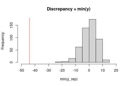
At this point, we can implement the check we want using our chosen discrepancy measure. Here a simple check uses the minimum observation.
obsMin <- min(data$y)
ppMin <- apply(ppSamples, 1, min)

# ## Check with plot in Gelman et al. (3rd edition), Figure 6.3
hist(ppMin, xlim = c(-50, 20),
    main = "Discrepancy = min(y)",
    xlab = "min(y_rep)")
abline(v = obsMin, col = 'red')
Fast posterior predictive sampling using a nimbleFunction
The approach above could be slow, even with a compiled model, because the loop is carried out in R. We could instead do all the work in a compiled nimbleFunction.
Writing the nimbleFunction
Let’s set up a nimbleFunction. In the setup code, we’ll manipulate the nodes and variables, similarly to the code above. In the run code, we’ll loop through the samples and simulate, also similarly.
Remember that all querying of the model structure needs to happen in the setup code. We also need to pass the MCMC object to the nimble function, so that we can determine at setup time the names of the variables we are copying from the posterior samples into the model.
The run code takes the actual samples as the input argument, so the nimbleFunction will work regardless of how long the MCMC was run for.
ppSamplerNF <- nimbleFunction(
          setup = function(model, mcmc) {
              dataNodes <- model$getNodeNames(dataOnly = TRUE)
              parentNodes <- model$getParents(dataNodes, stochOnly = TRUE)
              cat("Stochastic parents of data are:", paste(parentNodes, collapse = ','), ".\n")
              simNodes <- model$getDependencies(parentNodes, self = FALSE)
              vars <- mcmc$mvSamples$getVarNames()  # need ordering of variables in mvSamples / samples matrix
              cat("Using posterior samples of:", paste(vars, collapse = ','), ".\n")
              n <- length(model$expandNodeNames(dataNodes, returnScalarComponents = TRUE))
          },
          run = function(samples = double(2)) {
              nSamp <- dim(samples)[1]
              ppSamples <- matrix(nrow = nSamp, ncol = n)
              for(i in 1:nSamp) {
                    values(model, vars) <<- samples[i, ]
                    model$simulate(simNodes, includeData = TRUE)
                    ppSamples[i, ] <- values(model, dataNodes)
              }
              returnType(double(2))
              return(ppSamples)
          })
Using the nimbleFunction
We’ll create the instance of the nimbleFunction for this model and MCMC.
Then we run the compiled nimbleFunction.
## Create the sampler for this model and this MCMC.
ppSampler <- ppSamplerNF(model, mcmc)
## Stochastic parents of data are: mu,sigma .
## Using posterior samples of: mu,sigma .
cppSampler <- compileNimble(ppSampler, project = model)
## Check ordering of variables is same in 'vars' and in 'samples'.
colnames(samples)
## [1] "mu" "sigma"
identical(colnames(samples), model$expandNodeNames(mcmc$mvSamples$getVarNames()))
## [1] TRUE
set.seed(1)
system.time(ppSamples_via_nf <- cppSampler$run(samples))
##    user  system elapsed
##   0.004   0.000   0.004
identical(ppSamples, ppSamples_via_nf)
## [1] TRUE
So we get exactly the same results (note the use of set.seed to ensure this) but much faster.
Here the speed doesn’t really matter but for more samples and larger models it often will, even after accounting for the time spent to compile the nimbleFunction.
Version 0.11.1 of NIMBLE released
We’ve released the newest version of NIMBLE on CRAN and on our website. NIMBLE is a system for building and sharing analysis methods for statistical models, especially for hierarchical models and computationally-intensive methods (such as MCMC and SMC).
Version 0.11.1 is a bug fix release, fixing a bug that was introduced in Version 0.11.0 (which was released on April 17, 2021) that affected MCMC sampling in MCMCs using the “posterior_predictive_branch” sampler introduced in version 0.11.0. This sampler would be listed by name when the MCMC configuration object is created and would be assigned to any set of multiple nodes that (as a group of nodes) have no data dependencies and are therefore sampled as a group from their predictive distributions.
For those currently using version 0.11.0, please update your version of NIMBLE. For users currently using other versions, this release won’t directly affect you, but we generally encourage you to update as we release new versions.
Version 0.11.0 of NIMBLE released
- added the ‘posterior_predictive_branch’ MCMC sampler, which samples jointly from the predictive distribution of networks of entirely non-data nodes, to improve MCMC mixing,
- added a model method to find parent nodes, called getParents(), analogous to getDependencies(),
- improved efficiency of conjugate samplers,
- allowed use of the elliptical slice sampler for univariate nodes, which can be useful for posteriors with multiple modes,
- allowed model definition using if-then-else without an else clause, and
- fixed a bug giving incorrect node names and potentially affecting algorithm behavior for models with more than 100,000 elements in a vector node or any dimension of a multi-dimensional node.
Please see the release notes on our website for more details.
Bayesian Nonparametric Models in NIMBLE: General Multivariate Models
(Prepared by Claudia Wehrhahn)
Overview
NIMBLE is a hierarchical modeling package that uses nearly the same language for model specification as the popular MCMC packages WinBUGS, OpenBUGS and JAGS, while making the modeling language extensible — you can add distributions and functions — and also allowing customization of the algorithms used to estimate the parameters of the model.
NIMBLE supports Markov chain Monte Carlo (MCMC) inference for Bayesian nonparametric (BNP) mixture models. Specifically, NIMBLE provides functionality for fitting models involving Dirichlet process priors using either the Chinese Restaurant Process (CRP) or a truncated stick-breaking (SB) representation.
In version 0.10.1, we’ve extended NIMBLE to be able to handle more general multivariate models when using the CRP prior. In particular, one can now easily use the CRP prior when multiple observations (or multiple latent variables) are being jointly clustered. For example, in a longitudinal study, one may want to cluster at the individual level, i.e., to jointly cluster all of the observations for each of the individuals in the study. (Formerly this was only possible in NIMBLE by specifying the observations for each individual as coming from a single multivariate distribution.)
This allows one to specify a multivariate mixture kernel as the product of univariate ones. This is particularly useful when working with discrete data. In general, multivariate extensions of well-known univariate discrete distributions, such as the Bernoulli, Poisson and Gamma, are not straightforward. For example, for multivariate count data, a multivariate Poisson distribution might appear to be a good fit, yet its definition is not trivial, inference is cumbersome, and the model lacks flexibility to deal with overdispersion. See Inouye et al. (2017) for a review on multivariate distributions for count data based on the Poisson distribution.
In this post, we illustrate NIMBLE’s new extended BNP capabilities by modelling multivariate discrete data. Specifically, we show how to model multivariate count data from a longitudinal study under a nonparametric framework. The modeling approach is simple and introduces correlation in the measurements within subjects.
For more detailed information on NIMBLE and Bayesian nonparametrics in NIMBLE, see the User Manual.
BNP analysis of epileptic seizure count data
We illustrate the use of nonparametric multivariate mixture models for modeling counts of epileptic seizures from a longitudinal study of the drug progabide as an adjuvant antiepileptic chemotherapy. The data, originally reported in Leppik et al. (1985), arise from a clinical trial of 59 people with epilepsy. At four clinic visits, subjects reported the number of seizures occurring over successive two-week periods. Additional data include the baseline seizure count and the age of the patient. Patients were randomized to receive either progabide or a placebo, in addition to standard chemotherapy.
load(url("https://r-nimble.org/nimbleExamples/seizures.Rda"))
names(seizures)
## [1] "id" "seize" "visit" "trt" "age"
head(seizures)
##    id seize visit trt age
## 1 101    76     0   1  18
## 2 101    11     1   1  18
## 3 101    14     2   1  18
## 4 101     9     3   1  18
## 5 101     8     4   1  18
## 6 102    38     0   1  32
Model formulation
We model the joint distribution of the baseline number of seizures and the counts from each of the two-week periods as a Dirichlet Process mixture (DPM) of products of Poisson distributions. Let ")


where ")

, \quad\quad \boldsymbol{\lambda}_{i} \mid G \sim G, \quad\quad G \sim DP(\alpha, H),")
Our specification uses a product of Poisson distributions as the kernel in the DPM which, at first sight, would suggest independence of the repeated seizure count measurements. However, because we are mixing over the parameters, this specification in fact induces dependence within subjects, with the strength of the dependence being inferred from the data. In order to specify the model in NIMBLE, first we translate the information in seize into a matrix and then we write the NIMBLE code.
We specify this model in NIMBLE with the following code in R. The vector xi contains the latent cluster IDs, one for each patient.
n <- 59
J <- 5
data <- list(y = matrix(seizures$seize, ncol = J, nrow = n, byrow = TRUE))
constants <- list(n = n, J = J)

code <- nimbleCode({
  for(i in 1:n) {
    for(j in 1:J) {
      y[i, j] ~ dpois(lambda[xi[i], j])
    }
  }
  for(i in 1:n) {
    for(j in 1:J) {
      lambda[i, j] ~ dgamma(shape = 1, rate = 0.1)
    }
  }
  xi[1:n] ~ dCRP(conc = alpha, size = n)
  alpha ~ dgamma(shape = 1, rate = 1)
})
Running the MCMC
The following code sets up the data and constants, initializes the parameters, defines the model object, and builds and runs the MCMC algorithm. For speed, the MCMC runs using compiled C++ code, hence the calls to compileNimble to create compiled versions of the model and the MCMC algorithm.
Because the specification is in terms of a Chinese restaurant process, the default sampler selected by NIMBLE is a collapsed Gibbs sampler. More specifically, because the baseline distribution
set.seed(1)
inits <- list(xi = 1:n, alpha = 1,
             lambda = matrix(rgamma(J*n, shape = 1, rate = 0.1), ncol = J, nrow = n))
model <- nimbleModel(code, data=data, inits = inits, constants = constants, dimensions = list(lambda = c(n, J)))
cmodel <- compileNimble(model)
conf <- configureMCMC(model, monitors = c('xi','lambda', 'alpha'), print = TRUE)
## ===== Monitors =====
## thin = 1: xi, lambda, alpha
## ===== Samplers =====
## CRP_concentration sampler (1)
##   - alpha
## CRP_cluster_wrapper sampler (295)
##   - lambda[]  (295 elements)
## CRP sampler (1)
##   - xi[1:59]
mcmc <- buildMCMC(conf)
cmcmc <- compileNimble(mcmc, project = model)
samples <- runMCMC(cmcmc, niter=55000, nburnin = 5000, thin=10)
## |-------------|-------------|-------------|-------------|
## |-------------------------------------------------------|
We can extract posterior samples for some parameters of interest. The following are trace plots of the posterior samples for the concentration parameter, 
xiSamples <- samples[, grep('xi', colnames(samples))]    # samples of cluster IDs
nGroups <- apply(xiSamples, 1, function(x)  length(unique(x)))
concSamples <- samples[, grep('alpha', colnames(samples))]

par(mfrow=c(1, 2))
ts.plot(concSamples, xlab = "Iteration", ylab = expression(alpha), main = expression(paste('Traceplot for ', alpha)))
ts.plot(nGroups,  xlab = "Iteration", ylab = "Number of components", main = "Number of clusters")

Assessing the posterior
We can compute the posterior predictive distribution for a new observation 
")

")
# samples from the random measure
samplesG <- getSamplesDPmeasure(cmcmc)
niter <- length(samplesG)
weightsIndex <- grep('weights', colnames(samplesG[[1]]))
lambdaIndex <- grep('lambda', colnames(samplesG[[1]]))
ygrid <- 0:45

# function used to compute bivariate posterior predictive
bivariateFun <- nimbleFunction(
  run = function(w = double(1),
               lambda1 = double(1),
               lambda5 = double(1),
               ytilde = double(1)) {
    returnType(double(2))

    ngrid <- length(ytilde)
    out <- matrix(0, ncol = ngrid, nrow = ngrid)

    for(i in 1:ngrid) {
      for(j in 1:ngrid) {
        out[i, j] <- sum(w * dpois(ytilde[i], lambda1) * dpois(ytilde[j], lambda5))
      }
    }

    return(out)
  }
)
cbivariateFun <- compileNimble(bivariateFun)
# computing bivariate posterior predictive of seizure counts are baseline and fourth visit
bivariate <- matrix(0, ncol = length(ygrid), nrow = length(ygrid))
for(iter in 1:niter) {
  weights <- samplesG[[iter]][, weightsIndex] # posterior weights
  lambdaBaseline <- samplesG[[iter]][, lambdaIndex[1]] # posterior rate of baseline
  lambdaVisit4 <- samplesG[[iter]][, lambdaIndex[5]] # posterior rate at fourth visit
  bivariate <- bivariate + cbivariateFun(weights, lambdaBaseline, lambdaVisit4, ygrid)
}
bivariate <- bivariate / niter
The following code creates a heatmap of the posterior predictive bivariate distribution of the number of seizures at baseline and at the fourth hospital visit, showing that there is a positive correlation between these two measurements.
collist <- colorRampPalette(c('white', 'grey', 'black'))
image.plot(ygrid, ygrid, bivariate, col = collist(6),
           xlab = 'Baseline', ylab = '4th visit', ylim = c(0, 15), axes = TRUE)

In order to describe the uncertainty in the posterior clustering structure of the individuals in the study, we present a heat map of the posterior probability of two subjects belonging to the same cluster. To do this, first we compute the posterior pairwise clustering matrix that describes the probability of two individuals belonging to the same cluster, then we reorder the observations and finally plot the associated heatmap.
pairMatrix <- apply(xiSamples, 2, function(focal) {
                                   colSums(focal == xiSamples)
                                  })
pairMatrix <- pairMatrix / niter


newOrder <- c(1, 35, 13, 16, 32, 33,  2, 29, 39, 26, 28, 52, 17, 15, 23,  8, 31,
              38,  9, 46, 45, 11, 49, 44, 50, 41, 54, 21,  3, 40, 47, 48, 12,
              6, 14,  7, 18, 22, 30, 55, 19, 34, 56, 57,  4,  5, 58, 10, 43, 25,
              59, 20, 27, 24, 36, 37, 42, 51, 53)

reordered_pairMatrix <- pairMatrix[newOrder, newOrder]
image.plot(1:n, 1:n, reordered_pairMatrix , col = collist(6),
           xlab = 'Patient', ylab = 'Patient',  axes = TRUE)
axis(1, at = 1:n, labels = FALSE, tck = -.02)
axis(2, at = 1:n, labels = FALSE, tck = -.02)
axis(3, at = 1:n, tck = 0, labels = FALSE)
axis(4, at = 1:n, tck = 0, labels = FALSE)

References
Inouye, D.I., E. Yang, G.I. Allen, and P. Ravikumar. 2017. A Review of Multivariate Distributions for Count Data Derived from the Poisson Distribution. Wiley Interdisciplinary Reviews: Computational Statistics 9: e1398.
Leppik, I., F. Dreifuss, T. Bowman, N. Santilli, M. Jacobs, C. Crosby, J. Cloyd, et al. 1985. A Double-Blind Crossover Evaluation of Progabide in Partial Seizures: 3: 15 Pm8. Neurology 35.
Neal, R. 2000. Markov chain sampling methods for Dirichlet process mixture models. Journal of Computational and Graphical Statistics 9: 249–65.