Chapter 5 Writing models in NIMBLE’s dialect of BUGS
Models in NIMBLE are written using a variation on the BUGS language. From BUGS code, NIMBLE creates a model object. This chapter describes NIMBLE’s version of BUGS. The next chapter explains how to build and manipulate model objects.
5.1 Comparison to BUGS dialects supported by WinBUGS, OpenBUGS and JAGS
Many users will come to NIMBLE with some familiarity with WinBUGS, OpenBUGS, or JAGS, so we start by summarizing how NIMBLE is similar to and different from those before documenting NIMBLE’s version of BUGS more completely. In general, NIMBLE aims to be compatible with the original BUGS language and also JAGS’ version. However, at this point, there are some features not supported by NIMBLE, and there are some extensions that are planned but not implemented.
5.1.1 Supported features of BUGS and JAGS
- Stochastic and deterministic10 node declarations.
- Most univariate and multivariate distributions.
- Link functions.
- Most mathematical functions.
- ‘for’ loops for iterative declarations.
- Arrays of nodes up to 4 dimensions.
- Truncation and censoring as in JAGS using the
T()notation anddinterval.
5.1.2 NIMBLE’s Extensions to BUGS and JAGS
NIMBLE extends the BUGS language in the following ways:
- User-defined functions and distributions – written as nimbleFunctions – can be used in model code. See Chapter 12.
- Multiple parameterizations for distributions, similar to those in R, can be used.
- Named parameters for distributions and functions, similar to R function calls, can be used.
- Linear algebra, including for vectorized calculations of simple algebra, can be used in deterministic declarations.
- Distribution parameters can be expressions, as in JAGS but not in WinBUGS. Caveat: parameters to multivariate
distributions (e.g.,
dmnorm) cannot be expressions (but an expression can be defined in a separate deterministic expression and the resulting variable then used). - Alternative models can be defined from the same model code by using if-then-else statements that are evaluated when the model is defined.
- More flexible indexing of vector nodes within larger variables is allowed. For example one can place a multivariate normal vector arbitrarily within a higher-dimensional object, not just in the last index.
- More general constraints can be declared using
dconstraint, which extends the concept of JAGS’dinterval. - Link functions can be used in stochastic, as well as deterministic, declarations.11
- Data values can be reset, and which parts of a model are flagged as data can be changed, allowing one model to be used for different data sets without rebuilding the model each time.
- One can use stochastic/dynamic indexes, i.e., indexes can be other nodes or functions of other nodes. For a given dimension of a node being indexed, if the index is not constant, it must be a scalar value. So expressions such as
mu[k[i], 3]ormu[k[i], 1:3]ormu[k[i], j[i]]are allowed, but notmu[k[i]:(k[i]+1)]12 Nested dynamic indexes such asmu[k[j[i]]]are also allowed.
5.1.3 Not-supported features of BUGS and JAGS
The following are not supported.
- The appearance of the same node on the left-hand side of both a
<-and a \(\sim\) declaration (used in WinBUGS for data assignment for the value of a stochastic node). - Multivariate nodes must appear with brackets, even if they are
empty. E.g.,
xcannot be multivariate butx[]orx[2:5]can be. - NIMBLE generally determines the dimensionality and
sizes of variables from the BUGS code. However, when a variable
appears with blank indices, such as in
x.sum <- sum(x[]), and if the dimensions of the variable are not clearly defined in other declarations, NIMBLE currently requires that the dimensions of x be provided when the model object is created (vianimbleModel). - Use of non-sequential indexes in the definition of a for loop. JAGS allows syntax such as
for(i in expr)whenexprevaluates to an integer vector. In NIMBLE one can use the work-around of defining a constant vector, sayk, and usingk[i]in the body of the for loop. - Use of non-sequential indexes to subset variables. JAGS allows syntax such as
sum(mu[expr])whenexprevaluates to an integer vector. In NIMBLE one can use the work-around of defining a nimbleFunction that takesmuand the index vector as arguments and does the calculation of interest.
5.2 Writing models
Here we introduce NIMBLE’s version of BUGS. The WinBUGS, OpenBUGS and JAGS manuals are also useful resources for writing BUGS models, including many examples.
5.2.1 Declaring stochastic and deterministic nodes
BUGS is a declarative language for graphical (or hierarchical) models. Most programming languages are imperative, which means a series of commands will be executed in the order they are written. A declarative language like BUGS is more like building a machine before using it. Each line declares that a component should be plugged into the machine, but it doesn’t matter in what order they are declared as long as all the right components are plugged in by the end of the code.
The machine in this case is a graphical model13. A node (sometimes called a vertex) holds one value, which may be a scalar or a vector. Edges define the relationships between nodes. A huge variety of statistical models can be thought of as graphs.
Here is the code to define and create a simple linear regression model with four observations.
library(nimble)
mc <- nimbleCode({
    intercept ~ dnorm(0, sd = 1000)
    slope ~ dnorm(0, sd = 1000)
    sigma ~ dunif(0, 100)
    for(i in 1:4) {
        predicted.y[i] <- intercept + slope * x[i]
        y[i] ~ dnorm(predicted.y[i], sd = sigma)
    }
})

model <- nimbleModel(mc, data = list(y = rnorm(4)))

library(igraph)

layout <- matrix(ncol = 2, byrow = TRUE,
   # These seem to be rescaled to fit in the plot area,
   # so I'll just use 0-100 as the scale
                 data = c(33, 100,
                          66, 100,
                          50, 0, # first three are parameters
                          15, 50, 35, 50, 55, 50, 75, 50, # x's
                          20, 75, 40, 75, 60, 75, 80, 75, # predicted.y's
                          25, 25, 45, 25, 65, 25, 85, 25) # y's
                 )

sizes <- c(45, 30, 30,
           rep(20, 4),
           rep(50, 4),
           rep(20, 4))

edge.color <- "black"
    # c(
    # rep("green", 8),
    # rep("red", 4),
    # rep("blue", 4),
    # rep("purple", 4))
stoch.color <- "deepskyblue2"
det.color <- "orchid3"
rhs.color <- "gray73"
fill.color <- c(
    rep(stoch.color, 3),
    rep(rhs.color, 4),
    rep(det.color, 4),
    rep(stoch.color, 4)
)


plot(model$graph, vertex.shape = "crectangle",
     vertex.size = sizes,
     vertex.size2 = 20,
     layout = layout,
     vertex.label.cex = 3.0,
     vertex.color = fill.color,
     edge.width = 3,
     asp = 0.5,
     edge.color = edge.color)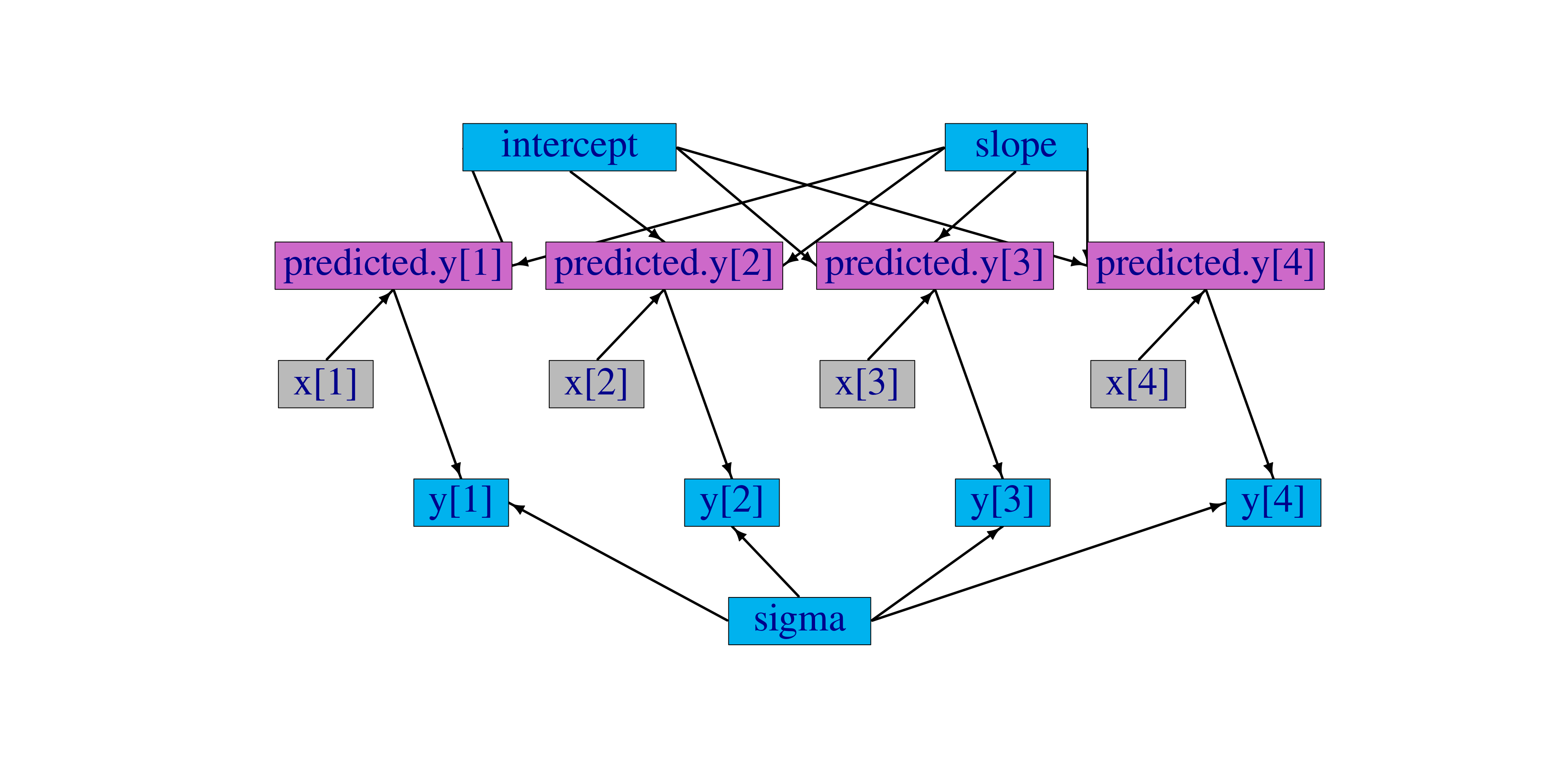
Figure 5.1: Graph of a linear regression model
The graph representing the model is
shown in Figure 5.1. Each observation,
y[i], is a node whose edges say that it follows a normal
distribution depending on a predicted value, predicted.y[i], and
standard deviation, sigma, which are each nodes. Each predicted
value is a node whose edges say how it is calculated from slope,
intercept, and one value of an explanatory variable, x[i],
which are each nodes.
This graph is created from the following BUGS code:
{
    intercept ~ dnorm(0, sd = 1000)
    slope ~ dnorm(0, sd = 1000)
    sigma ~ dunif(0, 100)
    for(i in 1:4) {
        predicted.y[i] <- intercept + slope * x[i]
        y[i] ~ dnorm(predicted.y[i], sd = sigma)
    }
}
In this code, stochastic relationships are declared with ‘\(\sim\)’
and deterministic relationships are declared with ‘<-’. For
example, each y[i] follows a normal distribution with mean
predicted.y[i] and standard deviation
sigma. Each
predicted.y[i] is the result of intercept + slope * x[i].
The for-loop yields the equivalent of writing four lines of code, each
with a different value of i. It does not matter in what order
the nodes are declared. Imagine that each line of code draws part of
Figure 5.1, and all that matters is that
the everything gets drawn in the end. Available distributions, default and alternative
parameterizations, and functions are listed in Section 5.2.4.
An equivalent graph can be created by this BUGS code:
{
    intercept ~ dnorm(0, sd = 1000)
    slope ~ dnorm(0, sd = 1000)
    sigma ~ dunif(0, 100)
    for(i in 1:4) {
        y[i] ~ dnorm(intercept + slope * x[i], sd = sigma)
    }
}
In this case, the predicted.y[i] nodes in Figure
5.1 will be created automatically by
NIMBLE and will have a different name, generated by NIMBLE.
5.2.2 More kinds of BUGS declarations
Here are some examples of valid lines of BUGS code. This code does
not describe a sensible or complete model, and it includes some
arbitrary indices (e.g. mvx[8:10, i]) to illustrate flexibility.
Instead the purpose of each line is to illustrate a feature of
NIMBLE’s version of BUGS.
{
    # 1. normal distribution with BUGS parameter order
    x ~ dnorm(a + b * c, tau)
    # 2. normal distribution with a named parameter
    y ~ dnorm(a + b * c, sd = sigma)
    # 3. For-loop and nested indexing
    for(i in 1:N) {
        for(j in 1:M[i]) {
            z[i,j] ~ dexp(r[ blockID[i] ])
        }
    }
    # 4. multivariate distribution with arbitrary indexing
    for(i in 1:3)
        mvx[8:10, i] ~ dmnorm(mvMean[3:5], cov = mvCov[1:3, 1:3, i])
    # 5. User-provided distribution
    w ~ dMyDistribution(hello = x, world = y)
    # 6. Simple deterministic node
    d1 <- a + b
    # 7. Vector deterministic node with matrix multiplication
    d2[] <- A[ , ] %*% mvMean[1:5]
    # 8. Deterministic node with user-provided function
    d3 <- foo(x, hooray = y)
}
When a variable appears only on the right-hand side, it can be provided via constants (in which case it can never be changed) or via data or inits, as discussed in Chapter 6.
Notes on the comment-numbered lines are:
xfollows a normal distribution with meana + b*cand precisiontau(default BUGS second parameter fordnorm).yfollows a normal distribution with the same mean asxbut a named standard deviation parameter instead of a precision parameter (sd = 1/sqrt(precision)).z[i, j]follows an exponential distribution with parameterr[ blockID[i] ]. This shows how for-loops can be used for indexing of variables containing multiple nodes. Variables that define for-loop indices (NandM) must also be provided as constants.
- The arbitrary block
mvx[8:10, i]follows a multivariate normal distribution, with a named covariance matrix instead of BUGS’ default of a precision matrix. As in R, curly braces for for-loop contents are only needed if there is more than one line. wfollows a user-defined distribution. See Chapter 12.d1is a scalar deterministic node that, when calculated, will be set toa + b.d2is a vector deterministic node using matrix multiplication in R’s syntax.d3is a deterministic node using a user-provided function. See Chapter 12.
5.2.2.1 More about indexing
Examples of allowed indexing include:
x[i]# a single indexx[i:j]# a range of indicesx[i:j,k:l]# multiple single indices or ranges for higher-dimensional arraysx[i:j, ]# blank indices indicating the full rangex[3*i+7]# computed indicesx[(3*i):(5*i+1)]# computed lower and upper ends of an index rangex[k[i]+1]# a dynamic (and computed) indexx[k[j[i]]]# nested dynamic indexesx[k[i], 1:3]# nested indexing of rows or columns
NIMBLE does not allow multivariate nodes to be used without
square brackets, which is an incompatibility with JAGS. Therefore a statement like xbar <- mean(x) in JAGS must be converted to
xbar <- mean(x[]) (if x is a vector) or xbar <- mean(x[,]) (if x is a matrix) for NIMBLE14. Section 6.1.1.5 discusses how to provide NIMBLE with dimensions of x when needed.
One cannot provide a vector of indices that are not constant. For example, x[start[i]:end[i]] is allowed only if start and end are provided as constants. Also, one cannot provide a vector, or expression evaluating to a vector (apart from use of :) as an index. For example, x[inds] is not allowed. Often one can write a nimbleFunction to achieve the desired result, such as definining a nimbleFunction that takes x, start[i], and end[i] or takes x and inds as arguments and does the subsetting (possibly in combination with some other calculation). Note that x[L:U] and x[inds] are allowed in nimbleFunction code.
Generally NIMBLE supports R-like linear algebra expressions and attempts to follow the same rules as R about
dimensions (although in some cases this is not possible). For
example, x[1:3] %*% y[1:3] converts x[1:3] into a row
vector and thus computes the inner product, which is returned as a \(1 \times 1\)
matrix (use inprod to get it as a scalar, which it typically easier). Like in R,
a scalar index will result in dropping a dimension unless the argument
drop=FALSE is provided. For example, mymatrix[i, 1:3] will
be a vector of length 3, but mymatrix[i, 1:3, drop=FALSE] will be
a \(1 \times 3\) matrix. More about indexing and dimensions is
discussed in Section 11.3.2.7.
5.2.3 Vectorized versus scalar declarations
Suppose you need nodes logY[i] that should be the log of the
corresponding Y[i], say for i from 1 to 10. Conventionally
this would be created with a for loop:
Since NIMBLE supports R-like algebraic expressions, an alternative in NIMBLE’s dialect of BUGS is to use a vectorized declaration like this:
There is an important difference between the models that are created by the
above two methods. The first creates 10 scalar nodes, logY[1]
\(,\ldots,\) logY[10]. The second creates one vector node,
logY[1:10]. If each logY[i] is used separately by an algorithm, it may be more efficient computationally if they are declared as scalars. If they are all used together,
it will often make sense to declare them as a vector.
5.2.4 Available distributions
5.2.4.1 Distributions
NIMBLE supports most of the distributions allowed in BUGS and JAGS. Table 5.1 lists the distributions that are currently supported, with their default parameterizations, which match those of BUGS15. NIMBLE also allows one to use alternative parameterizations for a variety of distributions as described next. See Section 12.2 to learn how to write new distributions using nimbleFunctions.
| Name | Usage | Density | Lower | Upper |
|---|---|---|---|---|
| Bernoulli | dbern(prob = p) |
\(p^x (1 - p)^{1 -x}\) | \(0\) | \(1\) |
| \(0 < p < 1\) | ||||
| Beta | dbeta(shape1 = a, |
\(\frac{x^{a-1}(1-x)^{b-1}}{\beta(a,b)}\) | \(0\) | \(1\) |
shape2 = b), \(a > 0\), \(b > 0\) |
||||
| Binomial | dbin(prob = p, size = n) |
\({n \choose x} p^x (1-p)^{n-x}\) | \(0\) | \(n\) |
| \(0 < p < 1\), \(n \in \mathbb{N}^*\) | ||||
| CAR | dcar_normal(adj, weights, |
see chapter 9 for details | ||
| (intrinsic) | num, tau, c, zero_mean) |
|||
| CAR | dcar_proper(mu, C, adj, |
see chapter 9 for details | ||
| (proper) | num, M, tau, gamma) |
|||
| Categorical | dcat(prob = p) |
\(\frac{p_x}{\sum_i p_i}\) | \(1\) | \(N\) |
| \(p \in (\mathbb{R}^+)^N\) | ||||
| Chi-square | dchisq(df = k), \(k > 0\) |
\(\frac{x^{\frac{k}{2}-1} \exp(-x/2)}{2^{\frac{k}{2}} \Gamma(\frac{k}{2})}\) | \(0\) | |
| Double | ddexp(location = \(\mu\), |
\(\frac{\tau}{2} \exp(-\tau |x - \mu|)\) | ||
| exponential | rate = \(\tau\)),\(\tau > 0\) |
|||
| Dirichlet | ddirch(alpha = \(\alpha\)) |
\(\Gamma(\sum_j \alpha_j) \prod_j \frac{ x_j^{\alpha_j - 1}}{ \Gamma(\alpha_j)}\) | \(0\) | |
| \(\alpha_j \geq 0\) | ||||
| Exponential | dexp(rate = \(\lambda\)), \(\lambda > 0\) |
\(\lambda \exp(-\lambda x)\) | \(0\) | |
| Flat | dflat() |
\(\propto 1\) (improper) | ||
| Gamma | dgamma(shape = r, rate = \(\lambda\)) |
\(\frac{ \lambda^r x^{r - 1} \exp(-\lambda x)}{ \Gamma(r)}\) | \(0\) | |
| \(\lambda > 0\), \(r > 0\) | ||||
| Half flat | dhalfflat() |
\(\propto 1\) (improper) | \(0\) | |
| Inverse | dinvgamma(shape = r, scale = \(\lambda\)) |
\(\frac{ \lambda^r x^{-(r + 1)} \exp(-\lambda / x)}{ \Gamma(r)}\) | \(0\) | |
| gamma | \(\lambda > 0\), \(r > 0\) | |||
| LKJ Correl’n | dlkj_corr_cholesky(eta = \(\eta\), |
\(\prod_{i=2}^{p} x_{ii}^{p - i + 2\eta -2}\) | ||
| Cholesky | size = p), \(\eta > 0\) |
|||
| Logistic | dlogis(location = \(\mu\), |
\(\frac{ \tau \exp\{(x - \mu) \tau\}}{\left[1 + \exp\{(x - \mu) \tau\}\right]^2}\) | ||
rate = \(\tau\)),\(\tau > 0\) |
||||
| Log-normal | dlnorm(meanlog = \(\mu\), |
\(\left(\frac{\tau}{2\pi}\right)^{\frac{1}{2}} x^{-1} \exp \left\{-\tau (\log(x) - \mu)^2 / 2 \right\}\) | \(0\) | |
taulog = \(\tau\)), \(\tau > 0\) |
||||
| Multinomial | dmulti(prob = p, size = n) |
\(n! \prod_j \frac{ p_j^{x_j}}{ x_j!}\) | ||
| \(\sum_j x_j = n\) | ||||
| Multivariate | dmnorm(mean = \(\mu\), prec = \(\Lambda\)) |
\((2\pi)^{-\frac{d}{2}}|\Lambda|^{\frac{1}{2}} \exp\{-\frac{(x-\mu)^T \Lambda (x-\mu)}{2}\}\) | ||
| normal | \(\Lambda\) positive definite | |||
| Multivariate | dmvt(mu = \(\mu\), prec = \(\Lambda\), |
\(\frac{\Gamma(\frac{\nu+d}{2})}{\Gamma(\frac{\nu}{2})(\nu\pi)^{d/2}}|\Lambda|^{1/2}(1+\frac{(x-\mu)^T\Lambda(x-\mu)}{\nu})^{-\frac{\nu+d}{2}}\) | ||
| Student t | df = \(\nu\)), \(\Lambda\) positive def. |
|||
| Negative | dnegbin(prob = p, size = r) |
\({x + r -1 \choose x} p^r (1-p)^x\) | \(0\) | |
| binomial | \(0 < p \leq 1\), \(r \geq 0\) | |||
| Normal | dnorm(mean = \(\mu\), tau = \(\tau\)) |
\(\left(\frac{\tau}{2\pi}\right)^{\frac{1}{2}} \exp\{- \tau (x - \mu)^2 / 2\}\) | ||
| \(\tau > 0\) | ||||
| Poisson | dpois(lambda = \(\lambda\)) |
\(\frac{ \exp(-\lambda)\lambda^x}{ x!}\) | \(0\) | |
| \(\lambda > 0\) | ||||
| Student t | dt(mu = \(\mu\), tau = \(\tau\), df = k) |
\(\frac{\Gamma(\frac{k+1}{2})}{\Gamma(\frac{k}{2})}\left(\frac{\tau}{k\pi}\right)^{\frac{1}{2}}\left\{1+\frac{\tau(x-\mu)^2}{k} \right\}^{-\frac{(k+1)}{2}}\) | ||
| \(\tau > 0\), \(k > 0\) | ||||
| Uniform | dunif(min = a, max = b) |
\(\frac{ 1}{ b - a}\) | \(a\) | \(b\) |
| \(a < b\) | ||||
| Weibull | dweib(shape = v, lambda = \(\lambda\)) |
\(v \lambda x^{v - 1} \exp (- \lambda x^v)\) | \(0\) | |
| \(v > 0\), \(\lambda > 0\) | ||||
| Wishart | dwish(R = R, df = k) |
\(\frac{ |x|^{(k-p-1)/2} |R|^{k/2} \exp\{-\text{tr}(Rx)/2\}}{ 2^{pk/2} \pi^{p(p-1)/4} \prod_{i=1}^{p} \Gamma((k+1-i)/2)}\) | ||
R \(p \times p\) pos. def., \(k \geq p\) |
||||
| Inverse | dinvwish(S = S, df = k) |
\(\frac{ |x|^{-(k+p+1)/2} |S|^{k/2} \exp\{-\text{tr}(Sx^{-1})/2\}}{ 2^{pk/2} \pi^{p(p-1)/4} \prod_{i=1}^{p} \Gamma((k+1-i)/2)}\) | ||
| Wishart | S \(p \times p\) pos. def., \(k \geq p\) |
5.2.4.1.1 Improper distributions
Note that dcar_normal, dflat and dhalfflat specify improper prior distributions
and should only be used when the posterior distribution of the model is known to be proper.
Also for these distributions, the density function returns the unnormalized density
and the simulation function returns NaN so these distributions
are not appropriate for algorithms that need to simulate from the
prior or require proper (normalized) densities.
5.2.4.1.2 LKJ distribution for correlation matrices
NIMBLE provides the LKJ distribution via dlkj_corr_cholesky
for correlation matrices, discussed in Section 24 of Stan Development Team (2021a) and based on
Lewandowski, Kurowicka, and Joe (2009). This distribution has various advantages (both from a modeling perspective and an
MCMC fitting perspective) over other prior distributions for correlation
or covariance matrices such as the inverse Wishart distribution.
For computational efficiency, the distribution is on the Cholesky factor of the correlation matrix rather than the correlation matrix itself. As a result using this distribution in a model involves a bit of care, including efficiently creating a covariance matrix from the correlation matrix and a set of standard deviations.
Here is some example code illustrating how to use the distribution in a model.
code <- nimbleCode({
    Ustar[1:p,1:p] ~ dlkj_corr_cholesky(1.3, p)
    U[1:p,1:p] <- uppertri_mult_diag(Ustar[1:p, 1:p], sds[1:p])
    for(i in 1:n)
        y[i, 1:p] ~ dmnorm(mu[1:p], cholesky = U[1:p, 1:p], prec_param = 0)
})
Note that we need to take the upper triangular Cholesky factor (Ustar) of the correlation matrix
and convert it to the upper triangular Cholesky factor (U) of a covariance matrix, based on a vector of
standard deviations (sds), and use that in the parameterization of
dmnorm that directly (and therefore efficiently) uses the Cholesky of the covariance.
Other approaches are possible, but unless care is taken they are likely to be less computationally efficient than the template above.
The template above uses a user-defined nimbleFunction to efficiently combine the Cholesky of the correlation matrix with a vector of standard deviations to produce the Cholesky of the covariance matrix. That function is given here:
uppertri_mult_diag <- nimbleFunction(
    run = function(mat = double(2), vec = double(1)) {
        returnType(double(2))
        p <- length(vec)
        out <- matrix(nrow = p, ncol = p, init = FALSE)
        for(i in 1:p)
            out[ , i] <- mat[ , i] * vec[i]
        return(out)
    })
Note that NIMBLE ignores the lower triangle of the Cholesky factor of the correlation matrix;
the values are taken to be zero. It also ignores the [1,1] element, which is taken to be one.
Any initial values for these elements will be ignored and simply repeated in the MCMC samples.
Assuming the [1,1] element is one and the lower triangle is filled with zeroes in the MCMC samples, one can
reconstruct a sample, here for the sth sample, of the correlation matrix as follows using the matrix of MCMC samples:
5.2.4.2 Alternative parameterizations for distributions
NIMBLE allows one to specify distributions in model code using a
variety of parameterizations, including the BUGS
parameterizations. Available parameterizations are listed in Table 5.2.
To understand how NIMBLE handles alternative parameterizations, it is
useful to distinguish three cases, using the gamma distribution
as an example:
- A canonical parameterization is used directly for
computations16. For
gamma, this is (shape, scale).
- The BUGS parameterization is the one defined in the
original BUGS language. In general this is the parameterization for which conjugate MCMC samplers can be executed most efficiently. For
dgamma, this is (shape, rate). - An alternative parameterization is one that must be
converted into the canonical parameterization. For
dgamma, NIMBLE provides both (shape, rate) and (mean, sd) parameterization and creates nodes to calculate (shape, scale) from either (shape, rate) or (mean, sd). In the case ofdgamma, the BUGS parameterization is also an alternative parameterization.
Since NIMBLE provides compatibility with existing BUGS and JAGS
code, the order of parameters places the BUGS parameterization
first. For example, the order of parameters for dgamma is dgamma(shape, rate, scale, mean, sd). Like R, if
parameter names are not given, they are taken in order, so that (shape,
rate) is the default. This happens to match R’s order of parameters,
but it need not. If names are given, they can be given in any
order. NIMBLE knows that rate is an alternative to scale and that
(mean, sd) are an alternative to (shape, scale or rate).
| Parameterization | NIMBLE re-parameterization |
|---|---|
dbern(prob) |
dbin(size = 1, prob) |
dbeta(shape1, shape2) |
canonical |
dbeta(mean, sd) |
dbeta(shape1 = mean^2 * (1-mean) / sd^2 - mean, |
shape2 = mean * (1 - mean)^2 / sd^2 + mean - 1) |
|
dbin(prob, size) |
canonical |
dcat(prob) |
canonical |
dchisq(df) |
canonical |
ddexp(location, scale) |
canonical |
ddexp(location, rate) |
ddexp(location, scale = 1 / rate) |
ddexp(location, var) |
ddexp(location, scale = sqrt(var / 2)) |
ddirch(alpha) |
canonical |
dexp(rate) |
canonical |
dexp(scale) |
dexp(rate = 1/scale) |
dgamma(shape, scale) |
canonical |
dgamma(shape, rate) |
dgamma(shape, scale = 1 / rate) |
dgamma(mean, sd) |
dgamma(shape = mean^2/sd^2, scale = sd^2/mean) |
dinvgamma(shape, rate) |
canonical |
dinvgamma(shape, scale) |
dgamma(shape, rate = 1 / scale) |
dlkj_corr_cholesky(eta) |
canonical |
dlogis(location, scale) |
canonical |
dlogis(location, rate) |
dlogis(location, scale = 1 / rate) |
dlnorm(meanlog, sdlog) |
canonical |
dlnorm(meanlog, taulog) |
dlnorm(meanlog, sdlog = 1 / sqrt(taulog)) |
dlnorm(meanlog, varlog) |
dlnorm(meanlog, sdlog = sqrt(varlog)) |
dmulti(prob, size) |
canonical |
dmnorm(mean, cholesky, |
canonical (precision) |
...prec_param=1) |
|
dmnorm(mean, cholesky, |
canonical (covariance) |
...prec_param=0) |
|
dmnorm(mean, prec) |
dmnorm(mean, cholesky = chol(prec), prec_param=1) |
dmnorm(mean, cov) |
dmnorm(mean, cholesky = chol(cov), prec_param=0) |
dmvt(mu, cholesky, df, |
canonical (precision/inverse scale) |
...prec_param=1) |
|
dmvt(mu, cholesky, df, |
canonical (scale) |
...prec_param=0) |
|
dmvt(mu, prec, df) |
dmvt(mu, cholesky = chol(prec), df, prec_param=1) |
dmvt(mu, scale, df) |
dmvt(mu, cholesky = chol(scale), df, prec_param=0) |
dlkj_corr_cholesky( |
canonical |
...shape, size) |
|
dnegbin(prob, size) |
canonical |
dnorm(mean, sd) |
canonical |
dnorm(mean, tau) |
dnorm(mean, sd = 1 / sqrt(var)) |
dnorm(mean, var) |
dnorm(mean, sd = sqrt(var)) |
dpois(lambda) |
canonical |
dt(mu, sigma, df) |
canonical |
dt(mu, tau, df) |
dt(mu, sigma = 1 / sqrt(tau), df) |
dt(mu, sigma2, df) |
dt(mu, sigma = sqrt(sigma2), df) |
dunif(min, max) |
canonical |
dweib(shape, scale) |
canonical |
dweib(shape, rate) |
dweib(shape, scale = 1 / rate) |
dweib(shape, lambda) |
dweib(shape, scale = lambda^(- 1 / shape)) |
dwish(cholesky, df, |
canonical (scale) |
...scale_param=1) |
|
dwish(cholesky, df, |
canonical (inverse scale) |
...scale_param=0) |
|
dwish(R, df) |
dwish(cholesky = chol(R), df, scale_param = 0) |
dwish(S, df) |
dwish(cholesky = chol(S), df, scale_param = 1) |
dinvwish(cholesky, df, |
canonical (scale) |
...scale_param=1) |
|
dinvwish(cholesky, df, |
canonical (inverse scale) |
...scale_param=0) |
|
dinvwish(R, df) |
dinvwish(cholesky = chol(R), df, scale_param = 0) |
dinvwish(S, df) |
dinvwish(cholesky = chol(S), df, scale_param = 1) |
Note that for multivariate normal, multivariate t, Wishart, and Inverse Wishart, the canonical
parameterization uses the Cholesky decomposition of one of the
precision/inverse scale or covariance/scale matrix. For example, for the multivariate normal, if prec_param=TRUE, the cholesky argument is treated as the Cholesky
decomposition of a precision matrix. Otherwise it is treated as the
Cholesky decomposition of a covariance matrix.
In addition, NIMBLE supports alternative distribution names, known as aliases, as in JAGS, as specified in Table 5.3.
| Distribution | Canonical name | Alias |
|---|---|---|
| Binomial | dbin | dbinom |
| Chi-square | dchisq | dchisqr |
| Double exponential | ddexp | dlaplace |
| Dirichlet | ddirch | ddirich |
| Multinomial | dmulti | dmultinom |
| Negative binomial | dnegbin | dnbinom |
| Weibull | dweib | dweibull |
| Wishart | dwish | dwishart |
We plan to, but do not currently, include the following distributions as part of core NIMBLE: beta-binomial, Dirichlet-multinomial, F, Pareto, or forms of the multivariate t other than the standard one provided.
5.2.5 Available BUGS language functions
Tables 5.4-5.5 show the available operators and functions. Support for more general R expressions is covered in Chapter 11 about programming with nimbleFunctions.
For the most part NIMBLE supports the functions used in BUGS and JAGS, with exceptions indicated in the table. Additional functions provided by NIMBLE are also listed. Note that we provide distribution functions for use in calculations, namely the ‘p’, ‘q’, and ‘d’ functions. See Section 11.2.4 for details on the syntax for using distribution functions as functions in deterministic calculations, as only some parameterizations are allowed and the names of some distributions differ from those used to define stochastic nodes in a model.
| Usage | Description | Comments | Status | Vector input |
|---|---|---|---|---|
x | y, x & y |
logical OR (\(|\)) and AND(&) | yes | yes | |
!x |
logical not | yes | yes | |
x > y, x >= y |
greater than (and or equal to) | yes | yes | |
x < y, x <= y |
less than (and or equal to) | yes | yes | |
x != y, x == y |
(not) equals | yes | yes | |
x + y, x - y, x * y |
component-wise operators | mix of scalar and vector | yes | yes |
x / y |
component-wise division | vector \(x\) and scalar \(y\) | yes | yes |
x^y, pow(x, y) |
power | \(x^y\); vector \(x\),scalar \(y\) | yes | yes |
x %% y |
modulo (remainder) | yes | no | |
min(x1, x2), |
min. (max.) of two scalars | yes | See pmin, |
|
max(x1, x2) |
pmax |
|||
exp(x) |
exponential | yes | yes | |
log(x) |
natural logarithm | yes | yes | |
sqrt(x) |
square root | yes | yes | |
abs(x) |
absolute value | yes | yes | |
step(x) |
step function at 0 | 0 if \(x<0\), 1 if \(x>=0\) | yes | yes |
equals(x, y) |
equality of two scalars | 1 if \(x==y\), 0 if \(x != y\) | yes | yes |
cube(x) |
third power | \(x^3\) | yes | yes |
sin(x), cos(x), |
trigonometric functions | yes | yes | |
tan(x) |
||||
asin(x), acos(x), |
inverse trigonometric functions | yes | yes | |
atan(x) |
||||
asinh(x), acosh(x), |
inv. hyperbolic trig. functions | yes | yes | |
atanh(x) |
||||
logit(x) |
logit | \(\log(x/(1-x))\) | yes | yes |
ilogit(x), expit(x) |
inverse logit | \(\exp(x)/(1 + \exp(x))\) | yes | yes |
probit(x) |
probit (Gaussian quantile) | \(\Phi^{-1}(x)\) | yes | yes |
iprobit(x), phi(x) |
inverse probit (Gaussian CDF) | \(\Phi(x)\) | yes | yes |
cloglog(x) |
complementary log log | \(\log(-\log(1-x))\) | yes | yes |
icloglog(x) |
inverse complementary log log | \(1 - \exp(-\exp(x))\) | yes | yes |
ceiling(x) |
ceiling function | \(\lceil(x)\rceil\) | yes | yes |
floor(x) |
floor function | \(\lfloor(x)\rfloor\) | yes | yes |
round(x) |
round to integer | yes | yes | |
trunc(x) |
truncation to integer | yes | yes | |
lgamma(x), loggam(x) |
log gamma function | \(\log \Gamma(x)\) | yes | yes |
besselK(x, nu, |
modified bessel function | returns vector even if | yes | yes |
...expon.scaled) |
of the second kind | \(x\) a matrix/array | ||
log1p(x) |
log of 1 + x | \(\log(1+x)\) | yes | yes |
lfactorial(x), |
log factorial | \(\log x!\) | yes | yes |
logfact(x) |
||||
qDIST(x, PARAMS) |
“q” distribution functions | canonical parameterization | yes | yes |
pDIST(x, PARAMS) |
“p” distribution functions | canonical parameterization | yes | yes |
rDIST(x, PARAMS) |
“r” distribution functions | canonical parameterization | yes | yes |
dDIST(x, PARAMS) |
“d” distribution functions | canonical parameterization | yes | yes |
sort(x) |
no | |||
rank(x, s) |
no | |||
ranked(x, s) |
no | |||
order(x) |
no |
| Usage | Description | Comments | Status |
|---|---|---|---|
inverse(x) |
matrix inverse | \(x\) symmetric, positive def. | yes |
chol(x) |
matrix Cholesky factorization | \(x\) symmetric, positive def. | yes |
| returns upper triang. matrix | |||
t(x) |
matrix transpose | \(x^\top\) | yes |
x%*%y |
matrix multiply | \(xy\); \(x\), \(y\) conformant | yes |
inprod(x, y) |
dot product | \(x^\top y\); \(x\) and \(y\) vectors | yes |
solve(x,y) |
solve system of equations | \(x^{-1} y\); \(y\) matrix or vector | yes |
forwardsolve(x, y) |
solve lower-triangular system of equations | \(x^{-1} y\); \(x\) lower-triangular | yes |
backsolve(x, y) |
solve upper-triangular system of equations | \(x^{-1} y\); \(x\) upper-triangular | yes |
logdet(x) |
log matrix determinant | \(\log|x|\) | yes |
asRow(x) |
convert vector to 1-row matrix | sometimes automatic | yes |
asCol(x) |
convert vector to 1-column matrix | sometimes automatic | yes |
sum(x) |
sum of elements of x |
yes | |
mean(x) |
mean of elements of x |
yes | |
sd(x) |
standard deviation of elements of x |
yes | |
prod(x) |
product of elements of x |
yes | |
min(x), max(x) |
min. (max.) of elements of x |
yes | |
pmin(x, y), pmax(x,y) |
vector of mins (maxs) of elements of | yes | |
x and y |
|||
interp.lin(x, v1, v2) |
linear interpolation | no | |
eigen(x)$values |
matrix eigenvalues | \(x\) symmetric | yes |
eigen(x)$vectors |
matrix eigenvectors | \(x\) symmetric | yes |
svd(x)$d |
matrix singular values | yes | |
svd(x)$u |
matrix left singular vectors | yes | |
svd(x)$v |
matrix right singular vectors | yes |
See Section 12.1 to learn how to use nimbleFunctions to write new functions for use in BUGS code.
5.2.6 Available link functions
NIMBLE allows the link functions listed in Table 5.6.
| Link function | Description | Range | Inverse |
|---|---|---|---|
cloglog(y) <- x |
Complementary log log | \(0 < y < 1\) | y <- icloglog(x) |
log(y) <- x |
Log | \(0 < y\) | y <- exp(x) |
logit(y) <- x |
Logit | \(0 < y < 1\) | y <- expit(x) |
probit(y) <- x |
Probit | \(0 < y < 1\) | y <- iprobit(x) |
Link functions are specified as functions applied to a node on the
left hand side of a BUGS expression. To handle link functions in
deterministic declarations, NIMBLE converts the declaration into an
equivalent inverse declaration. For example, log(y) <- x is
converted into y <- exp(x). In other words, the link function is
just a simple variant for conceptual clarity.
To handle link functions in a stochastic declaration, NIMBLE
does some processing that inserts an additional node into the model.
For example, the declaration logit(p[i]) ~ dnorm(mu[i],1), is equivalent
to the following two declarations:
logit_p[i] ~ dnorm(mu[i], 1),p[i] <- expit(logit_p[i])
where expit is the inverse of logit.
Note that NIMBLE does not provide an automatic way of initializing the additional node (logit_p[i] in this case), which is a parent node of the explicit node (p[i]), without explicitly referring to the additional node by the name that NIMBLE generates.
5.2.7 Truncation, censoring, and constraints
NIMBLE provides three ways to declare boundaries on the value of a variable, each for different situations. We introduce these and comment on their relationships to related features of JAGS and BUGS. The three methods are:
5.2.7.1 Truncation
Either of the following forms,
x ~ dnorm(0, sd = 10) T(0, a)
x ~ T(dnorm(0, sd = 10), 0, a)
declares that x follows a normal distribution between 0 and
a (inclusive of 0 and a). Either boundary may be omitted or may be another node, such as a in this example. The first form is compatible with JAGS, but in NIMBLE it can only be used when reading code from a text file. When writing model code in R, the second version must be used.
Truncation means the possible values of x are limited a priori, hence the probability density of x must be normalized17. In this example it would be the normal probability density divided by its integral from 0 to a. Like JAGS, NIMBLE also provides I as a synonym for T to accommodate older BUGS code, but T is preferred because it disambiguates multiple usages of I in BUGS.
5.2.7.2 Censoring
Censoring refers to the situation where one datum gives the lower or upper bound on an unobserved random variable. This is common in survival analysis, when for an individual still surviving at the end of a study, the age of death is not known and hence is ‘censored’ (right-censoring). NIMBLE adopts JAGS syntax for censoring, as follows:
In the case of right-censoring, censored[i] should be given as data with a value of 1 if
t[i] is right-censored (t[i] > c[i]) and 0 if it is
observed. The data vector for t should have NA (indicating
missing data) for any censored t[i] entries. (As a result, these
nodes will be sampled in an MCMC.) The vector for c should
give the censoring times corresponding to censored entries and a value
above the observed times for uncensored entries (e.g., Inf). The values for c
can be provided via constants, inits, or data. We recommend providing
via constants for values that are fixed and via inits for values that are
to be estimated or might be changed for some reason.
Left-censored observations would be specified by setting censored[i] to 0
and t[i] to NA.
Important: The value of t[i] corresponding to each censored data point should be given a
valid initial value (via inits) that is consistent with censored[i]. Otherwise, NIMBLE will initialize
from the prior, which may not produce a valid initial value.
The dinterval is not really a distribution but rather a trick: in the above example when censored[i] = 1 it gives a ‘probability’ of 1 if t[i] > c[i] and 0 otherwise. This means that t[i] <= c[i] is treated as impossible. More generally than simple right- or left-censoring, censored[i] ~ dinterval(t[i], c[i, ]) is defined such that for a vector of increasing cutpoints, c[i, ], t[i] is enforced to fall within the censored[i]-th cutpoint interval. This is done by setting data censored[i] as follows:
censored[i] = 0 if t[i] <= c[i, 1]
censored[i] = m if c[i, m] < t[i] <= c[i, m+1] for \(1 \leq m \leq M\)
censored[i] = M if c[i, M] < t[i]
(The i index is provided only for consistency with the previous example.) The most common uses of dinterval will be for left- and right-censored data, in which case c[i,] will be a single value (and typically given as simply c[i]), and for interval-censored data, in which case c[i,] will be a vector of two values.
Nodes following a dinterval distribution should normally be set
as data with known values. Otherwise, the node may be simulated during initialization in some algorithms (e.g., MCMC) and thereby establish a permanent, perhaps unintended, constraint.
Censoring differs from truncation because censoring an observation involves bounds on a random variable that could have taken any value, while in truncation we know a priori that a datum could not have occurred outside the truncation range.
5.2.7.3 Constraints and ordering
NIMBLE provides a more general way to enforce constraints using dconstraint(cond). For example, we could specify that the sum of mu1 and mu2 must be positive like this:
with constraint_data set (as data) to 1. This is
equivalent to a half-normal distribution on the half-plane \(\mu_1 +
\mu_2 > 0\). Nodes following dconstraint should be provided as data for the same reason of avoiding unintended initialization described above for dinterval.
Important: the model should be initialized so that the constraints are satisfied. Otherwise, NIMBLE will initialize from the prior, which may not produce a valid initial value and may cause algorithms (particularly) MCMC to fail.
Formally, dconstraint(cond) is a probability distribution on \(\left\{ 0, 1 \right\}\) such that \(P(1) = 1\) if cond is TRUE and \(P(0) = 1\) if cond is FALSE.
Of course, in many cases, parameterizing the model so that the
constraints are automatically respected may be a better strategy than
using dconstraint. One should be cautious about constraints that
would make it hard for an MCMC or optimization to move through the
parameter space (such as equality constraints that involve two or more
parameters). For such restrictive constraints, general purpose
algorithms that are not tailored to the constraints may fail or be inefficient. If constraints are used, it will generally be wise to ensure the model is initialized with values that satisfy them.
5.2.7.3.1 Ordering
To specify an ordering of parameters, such as \(\alpha_1 <= \alpha_2 <= \alpha_3\) one can use dconstraint as follows:
Note that unlike in BUGS, one cannot specify prior ordering using syntax such as
alpha[1] ~ dnorm(0, 1) I(, alpha[2])
alpha[2] ~ dnorm(0, 1) I(alpha[1], alpha[3])
alpha[3] ~ dnorm(0, 1) I(alpha[2], )
as this does not represent a directed acyclic graph.
Also note that specifying prior ordering using T(,) can result in possibly unexpected results. For example:
will enforce alpha1 \(\le\) alpha2 \(\le\) alpha3, but it does not treat the three parameters symmetrically. Instead it puts a marginal prior on alpha1 that is standard normal and then constrains alpha2 and alpha3 to follow truncated normal distributions. This is not equivalent to a symmetric prior on the three alphas that assigns zero probability density when values are not in order.
NIMBLE does not support the JAGS sort syntax.
5.2.8 Model macros
A NIMBLE macro is a succinct syntax that expands to create the NIMBLE model code for part or all of a model.
The nimbleMacros package provides an initial set of macros, currently focused on linear modeling and include:
LM: specify a complete generalized linear model (GLM) or generalized linear mixed model (GLMM), using standard R andlme4model formula syntax,LINPRED: specify a linear predictor using a standard R formula,FORLOOP: specify a for loop by providing code with index ranges.
These macros are discussed in detail in the vignette for the nimbleMacros package and in the documentation for each macro, e.g., help(LINPRED).
Here is a brief example of using the LM macro to set up a GLMM.
We’ll consider the Chick example from the lme4 package. We’ll set up a NIMBLE model analogous to this mixed effects model specified with lme4::lmer:
with a linear effect of time and random intercepts for each chick.
Here’s the specification of the model code in nimble, using the LM macro:
library(nimbleMacros)

code <- nimbleCode({
  LM(weight[1:N] ~ Time + (1|Chick))
})

chickConst <- list(Time = ChickWeight$Time, Chick = ChickWeight$Chick,
                    N = nrow(ChickWeight))
chickData <- list(weight = ChickWeight$weight)

mod <- nimbleModel(code, constants = chickConst, data = chickData)

mod$getCode()
## {
## "# LM"
## " ## FORLOOP"
## for (i_1 in 1:N) {
## weight[i_1] ~ dnorm(mu_[i_1], sd = sd_residual)
## }
## " ## ----"
## " ## LINPRED"
## " ### nimbleMacros::FORLOOP"
## for (i_2 in 1:N) {
## mu_[i_2] <- beta_Intercept + beta_Time * Time[i_2] +
## beta_Chick[Chick[i_2]]
## }
## " ### ----"
## " ### nimbleMacros::LINPRED_PRIORS"
## beta_Intercept ~ dnorm(0, sd = 1000)
## beta_Time ~ dnorm(0, sd = 1000)
## sd_Chick ~ dunif(0, 100)
## " #### nimbleMacros::FORLOOP"
## for (i_3 in 1:50) {
## beta_Chick[i_3] ~ dnorm(0, sd = sd_Chick)
## }
## " #### ----"
## " ### ----"
## " ## ----"
## sd_residual ~ dunif(0, 100)
## "# ----"
## }We can see list of the names of the model variables created by macros in the model using the getMacroParameters() function:
## $LM
## $LM[[1]]
## [1] "mu_"         "sd_residual"
##
##
## $FORLOOP
## $FORLOOP[[1]]
## NULL
##
##
## $LINPRED
## $LINPRED[[1]]
## [1] "beta_Intercept" "beta_Time"      "beta_Chick"
##
##
## $`nimbleMacros::FORLOOP`
## $`nimbleMacros::FORLOOP`[[1]]
## NULL
##
## $`nimbleMacros::FORLOOP`[[2]]
## NULL
##
##
## $`nimbleMacros::LINPRED_PRIORS`
## $`nimbleMacros::LINPRED_PRIORS`[[1]]
## [1] "beta_Intercept" "beta_Time"      "sd_Chick"       "beta_Chick"
That specified the entire model with a macro. One can also use macros to create the code for components of a model. Here’s a brief example.
Here’s a complete linear regression model (in this example omitting the random effects) of chick weight as a function of time making use of LINPRED and FORLOOP (similar to the code generated by LM):
code <- nimbleCode({
  mu[1:N] <- LINPRED(~Time[1:N])

  weight[1:N] ~ FORLOOP(dnorm(mu[1:N], sd = sigma))
  sigma ~ dunif(0, 100)
})
mod <- nimbleModel(code, constants = chickConst, data = chickData)
mod$getCode()
## {
## "# LINPRED"
## " ## nimbleMacros::FORLOOP"
## for (i_1 in 1:N) {
## mu[i_1] <- beta_Intercept + beta_Time * Time[i_1]
## }
## " ## ----"
## " ## nimbleMacros::LINPRED_PRIORS"
## beta_Intercept ~ dnorm(0, sd = 1000)
## beta_Time ~ dnorm(0, sd = 1000)
## " ## ----"
## "# ----"
## "# FORLOOP"
## for (i_2 in 1:N) {
## weight[i_2] ~ dnorm(mu[i_2], sd = sigma)
## }
## "# ----"
## sigma ~ dunif(0, 100)
## }As discussed in Section 12.4, NIMBLE users can also create new macros to use in models.
NIMBLE calls non-stochastic nodes ‘deterministic’, whereas BUGS calls them ‘logical’. NIMBLE uses ‘logical’ in the way R does, to refer to boolean (TRUE/FALSE) variables.↩︎
But beware of the possibility of needing to set values for ‘lifted’ nodes created by NIMBLE.↩︎
In some cases, one can write a nimbleFunction to achieve the desired result, such as replacing
sum(mu[start[i]:end[i]])with a nimbleFunction that takesmu,start[i], andend[i]as arguments and does the needed summation.↩︎Technically, a directed acyclic graph↩︎
In
nimbleFunctions, as explained in later chapters, square brackets with blank indices are not necessary for multivariate objects.↩︎Note that the same distributions are available for writing
nimbleFunctions, but in that case the default parameterizations and function names match R’s when possible. Please see Section 11.2.4 for how to use distributions innimbleFunctions.↩︎Usually this is the parameterization in the
Rmathheader of R’s C implementation of distributions.↩︎NIMBLE uses the CDF and inverse CDF (quantile) functions of a distribution to do this; in some cases if one uses truncation to include only the extreme tail of a distribution, numerical difficulties can arise.↩︎