Bayesian nonparametrics in NIMBLE: Nonparametric random effects
Overview
NIMBLE is a hierarchical modeling package that uses nearly the same language for model specification as the popular MCMC packages WinBUGS, OpenBUGS and JAGS, while making the modeling language extensible — you can add distributions and functions — and also allowing customization of the algorithms used to estimate the parameters of the model.
Recently, we added support for Markov chain Monte Carlo (MCMC) inference for Bayesian nonparametric (BNP) mixture models to NIMBLE. In particular, starting with version 0.6-11, NIMBLE provides functionality for fitting models involving Dirichlet process priors using either the Chinese Restaurant Process (CRP) or a truncated stick-breaking (SB) representation of the Dirichlet process prior.
We will illustrate NIMBLE’s BNP capabilities using two examples. In a previous post, we showed how to use nonparametric mixture models with different kernels for density estimation. In this post, we will take a parametric generalized linear mixed model and show how to switch to a nonparametric representation of the random effects that avoids the assumption of normally-distributed random effects.
For more detailed information on NIMBLE and Bayesian nonparametrics in NIMBLE, see the NIMBLE User Manual.
Parametric meta analysis of Avandia myocardial infarctions (MIs)
We will illustrate the use of nonparametric mixture models for modeling random effects distributions in the context of a meta-analysis of the side effects of a formerly very popular drug for diabetes called Avandia. The data we analyze played a role in raising serious questions about the safety of this drug. The question is whether Avandia use increases the risk of myocardial infarction (heart attack). There are 48 studies (the 49th study in the data file is different in some ways and excluded here), each with treatment and control arms.
dat <- read.csv('https://rawgit.com/nimble-dev/nimble-demos/master/intro_bnp/avandia.csv')
head(dat)
## trial nAvandia avandiaMI nControl controlMI
## 1 1 357 2 176 0
## 2 2 391 2 207 1
## 3 3 774 1 185 1
## 4 4 213 0 109 1
## 5 5 232 1 116 0
## 6 6 43 0 47 1
Model formulation
We begin with a standard generalized linear mixed model (GLMM)-based meta analysis. The vectors  and
and  contain the total number of patients in the control and the number of patients suffering from myocardial infarctions in the control group of each study, respectively. Similarly, the vectors
  and
and  contain similar information for patients receiving the drug Avandia. The model takes the form
 , \quad\quad y_{i} \mid \theta, \gamma_i \sim \mbox{Bin} \left(m_i, \frac{\exp\left\{ \theta + \gamma_i \right\}}{1 + \exp\left\{ \theta + \gamma_i \right\}} \right)")
where the random effects,  , follow a common normal distribution,
 ") , and the
, and the  and
and  are given reasonably non-informative priors. The parameter quantifies the difference in risk between the control and treatment arms, while the quantify study-specific variation.
This model can be specified in NIMBLE using the following code:
x <- dat$controlMI
n <- dat$nControl
y <- dat$avandiaMI
m <- dat$nAvandia
nStudies <- nrow(dat)
data <- list(x = x, y = y)
constants = list(n = n, m = m, nStudies = nStudies)
codeParam <- nimbleCode({
for(i in 1:nStudies) {
y[i] ~ dbin(size = m[i], prob = q[i]) # avandia MIs
x[i] ~ dbin(size = n[i], prob = p[i]) # control MIs
q[i] <- expit(theta + gamma[i]) # Avandia log-odds
p[i] <- expit(gamma[i]) # control log-odds
gamma[i] ~ dnorm(mu, var = tau2) # study effects
}
theta ~ dflat() # effect of Avandia
# random effects hyperparameters
mu ~ dnorm(0, 10)
tau2 ~ dinvgamma(2, 1)
})
Running the MCMC
Let’s run a basic MCMC.
set.seed(9)
inits = list(theta = 0, mu = 0, tau2 = 1, gamma = rnorm(nStudies))
samples <- nimbleMCMC(code = codeParam, data = data, inits = inits,
constants = constants, monitors = c("mu", "tau2", "theta", "gamma"),
thin = 10, niter = 22000, nburnin = 2000, nchains = 1, setSeed = TRUE)
## setting data and initial values...
## running calculate on model (any error reports that follow may simply reflect missing values in model variables) ...
## checking model sizes and dimensions...
## checking model calculations...
## model building finished.
## compiling... this may take a minute. Use 'showCompilerOutput = TRUE' to see C++ compiler details.
## compilation finished.
## runMCMC's handling of nburnin changed in nimble version 0.6-11. Previously, nburnin samples were discarded *post-thinning*. Now nburnin samples are discarded *pre-thinning*. The number of samples returned will be floor((niter-nburnin)/thin).
## running chain 1...
## |-------------|-------------|-------------|-------------|
## |-------------------------------------------------------|
par(mfrow = c(1, 4), cex = 1.1, mgp = c(1.8,.7,0))
ts.plot(samples[ , 'theta'], xlab = 'iteration', ylab = expression(theta))
hist(samples[ , 'theta'], xlab = expression(theta), main = 'effect of Avandia')
gammaCols <- grep('gamma', colnames(samples))
gammaMn <- colMeans(samples[ , gammaCols])
hist(gammaMn, xlab = 'posterior means', main = 'random effects distribution')
hist(samples[1000, gammaCols], xlab = 'single draw',
main = 'random effects distribution')
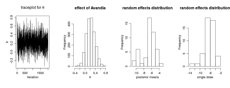
The results suggests there is an overall difference in risk between the control and treatment arms. But what about the normality assumption? Are our conclusions robust to that assumption? Perhaps the random effects distribution are skewed. (And recall that the estimates above of the random effects are generated under the normality assumption, which pushes the estimated effects to look more normal…)
DP-based random effects modeling for meta analysis
Model formulation
Now, we use a nonparametric distribution for the s. More specifically, we assume that each is generated from a location-scale mixture of normal distributions:
, \quad\quad (\mu_i, \tau_i^2) \mid G \sim G, \quad\quad G \sim \mbox{DP}(\alpha, H),")
where  is a normal-inverse-gamma distribution.
This specification induces clustering among the random effects. As in the case of density estimation problems, the DP prior allows the data to determine the number of components, from as few as one component (i.e., simplifying to the parametric model), to as many as components, i.e., one component for each observation. This allows the distribution of the random effects to be multimodal if the data supports such behavior, greatly increasing its flexibility. This model can be specified in NIMBLE using the following code:
Running the MCMC
The following code compiles the model and runs a collapsed Gibbs sampler for the model
inits <- list(gamma = rnorm(nStudies), xi = sample(1:2, nStudies, replace = TRUE),
alpha = 1, mu0 = 0, var0 = 1, a0 = 1, b0 = 1, theta = 0,
muTilde = rnorm(nStudies), tau2Tilde = rep(1, nStudies))
samplesBNP <- nimbleMCMC(code = codeBNP, data = data, inits = inits,
constants = constants,
monitors = c("theta", "gamma", "alpha", "xi", "mu0", "var0", "a0", "b0"),
thin = 10, niter = 22000, nburnin = 2000, nchains = 1, setSeed = TRUE)
## setting data and initial values...
## running calculate on model (any error reports that follow may simply reflect missing values in model variables) ...
## checking model sizes and dimensions...
## checking model calculations...
## model building finished.
## compiling... this may take a minute. Use 'showCompilerOutput = TRUE' to see C++ compiler details.
## compilation finished.
## runMCMC's handling of nburnin changed in nimble version 0.6-11. Previously, nburnin samples were discarded *post-thinning*. Now nburnin samples are discarded *pre-thinning*. The number of samples returned will be floor((niter-nburnin)/thin).
## running chain 1...
## |-------------|-------------|-------------|-------------|
## |-------------------------------------------------------|
gammaCols <- grep('gamma', colnames(samplesBNP))
gammaMn <- colMeans(samplesBNP[ , gammaCols])
xiCols <- grep('xi', colnames(samplesBNP))

par(mfrow = c(1,5), cex = 1.1, mgp = c(1.8,.7,0))
ts.plot(samplesBNP[ , 'theta'], xlab = 'iteration', ylab = expression(theta),
   main = expression(paste('traceplot for ', theta)))
hist(samplesBNP[ , 'theta'], xlab = expression(theta), main = 'effect of Avandia')
hist(gammaMn, xlab = 'posterior means',
              main = "random effects distrib'n")
hist(samplesBNP[1000, gammaCols], xlab = 'single draw',
                   main = "random effects distrib'n")

# How many mixture components are inferred?
xiRes <- samplesBNP[ , xiCols]
nGrps <- apply(xiRes, 1, function(x) length(unique(x)))
ts.plot(nGrps, xlab = 'iteration', ylab = 'number of components',
   main = 'number of components')
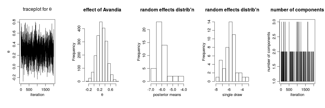
The primary inference seems robust to the original parametric assumption. This is probably driven by the fact that there is not much evidence of lack of normality in the random effects distribution (as evidenced by the fact that the posterior distribution of the number of mixture components places a large amount of probability on exactly one component).
More information and future development
Please see our User Manual for more details.
We’re in the midst of improvements to the existing BNP functionality as well as adding additional Bayesian nonparametric models, such as hierarchical Dirichlet processes and Pitman-Yor processes, so please add yourself to our announcement or user support/discussion Google groups.