One nice feature of NIMBLE’s MCMC system is that a user can easily write new samplers from R, combine them with NIMBLE’s samplers, and have them automatically compiled to C++ via the NIMBLE compiler. We’ve observed that block sampling using a simple adaptive multivariate random walk Metropolis-Hastings sampler doesn’t always work well in practice, so we decided to implement the Automated Factor Slice sampler (AFSS) of Tibbits, Groendyke, Haran, and Liechty (2014) and see how it does on a (somewhat artificial) example with severe posterior correlation problems.
Roughly speaking, the AFSS works by conducting univariate slice sampling in directions determined by the eigenvectors of the marginal posterior covariance matrix for blocks of parameters in a model. So far, we’ve found the AFSS often outperforms random walk block sampling. To compare performance, we look at MCMC efficiency, which we define for each parameter as effective sample size (ESS) divided by computation time. We define overall MCMC efficiency as the minimum MCMC efficiency of all the parameters, because one needs all parameters to be well mixed.
We’ll demonstrate the performance of the AFSS on the correlated state space model described in Turek, de.
Valpine, Paciorek, Anderson-Bergman, and others (2017)
Model Creation
Assume 


")
")
for 
")
")
and prior distributions
")
")
")
")
where ")


A file named model_SSMcorrelated.RData with the BUGS model code, data, constants, and initial values for our model can be downloaded here.
## load the nimble library and set seed
library('nimble')
set.seed(1)
load('model_SSMcorrelated.RData')
## build and compile the model
stateSpaceModel <- nimbleModel(code = code,
                              data = data,
                              constants = constants,
                              inits = inits,
                              check = FALSE)

C_stateSpaceModel <- compileNimble(stateSpaceModel)
Comparing two MCMC Samplers
We next compare the performance of two MCMC samplers on the state space model described above. The first sampler we consider is NIMBLE’s RW_block sampler, a Metropolis-Hastings sampler with a multivariate normal proposal distribution. This sampler has an adaptive routine that modifies the proposal covariance to look like the empirical covariance of the posterior samples of the parameters. However, as we shall see below, this proposal covariance adaptation does not lead to efficient sampling for our state space model.
We first build and compile the MCMC algorithm.
RW_mcmcConfig <- configureMCMC(stateSpaceModel)
RW_mcmcConfig$removeSamplers(c('a', 'b', 'sigOE', 'sigPN'))
RW_mcmcConfig$addSampler(target = c('a', 'b', 'sigOE', 'sigPN'), type = 'RW_block')
RW_mcmc <- buildMCMC(RW_mcmcConfig)
C_RW_mcmc <- compileNimble(RW_mcmc, project = stateSpaceModel)
We next run the compiled MCMC algorithm for 10,000 iterations, recording the overall MCMC efficiency from the posterior output. The overall efficiency here is defined as ")

RW_minEfficiency <- numeric(5)
for(i in 1:5){
  runTime <- system.time(C_RW_mcmc$run(50000, progressBar = FALSE))['elapsed']
  RW_mcmcOutput <- as.mcmc(as.matrix(C_RW_mcmc$mvSamples))
  RW_minEfficiency[i] <- min(effectiveSize(RW_mcmcOutput)/runTime)
}
summary(RW_minEfficiency)
##    Min. 1st Qu.  Median    Mean 3rd Qu.    Max.
##  0.3323  0.4800  0.5505  0.7567  0.7341  1.6869
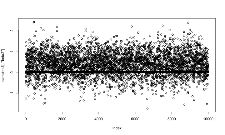
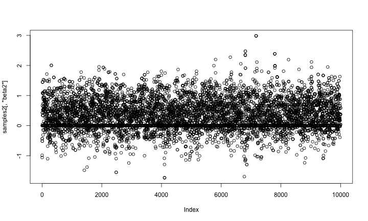
Examining a trace plot of the output below, we see that the $a$ and $b$ parameters are mixing especially poorly.
plot(RW_mcmcOutput, density = FALSE)

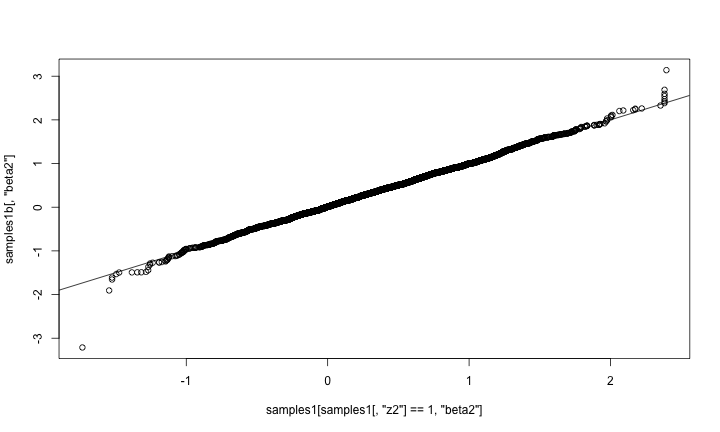
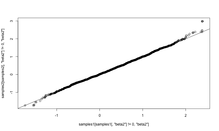
Plotting the posterior samples of 

plot.default(RW_mcmcOutput[,'a'], RW_mcmcOutput[,'b'])

cor(RW_mcmcOutput[,'a'], RW_mcmcOutput[,'b'])
## [1] -0.9201277
In such situations with strong posterior correlation, we’ve found the AFSS to often run much more efficiently, so we next build and compile an MCMC algorithm using the AFSS sampler. Our hope is that the AFSS sampler will be better able to to produce efficient samples in the face of high posterior correlation.
AFSS_mcmcConfig <- configureMCMC(stateSpaceModel)
AFSS_mcmcConfig$removeSamplers(c('a', 'b', 'sigOE', 'sigPN'))
AFSS_mcmcConfig$addSampler(target = c('a', 'b', 'sigOE', 'sigPN'), type = 'AF_slice')
AFSS_mcmc<- buildMCMC(AFSS_mcmcConfig)
C_AFSS_mcmc <- compileNimble(AFSS_mcmc, project = stateSpaceModel, resetFunctions = TRUE)
We again run the AFSS MCMC algorithm 5 times, each with 10,000 MCMC iterations.
AFSS_minEfficiency <- numeric(5)
for(i in 1:5){
  runTime <- system.time(C_AFSS_mcmc$run(50000, progressBar = FALSE))['elapsed']
  AFSS_mcmcOutput <- as.mcmc(as.matrix(C_AFSS_mcmc$mvSamples))
  AFSS_minEfficiency[i] <- min(effectiveSize(AFSS_mcmcOutput)/runTime)
}
summary(AFSS_minEfficiency)
##    Min. 1st Qu.  Median    Mean 3rd Qu.    Max.
##   9.467   9.686  10.549  10.889  10.724  14.020
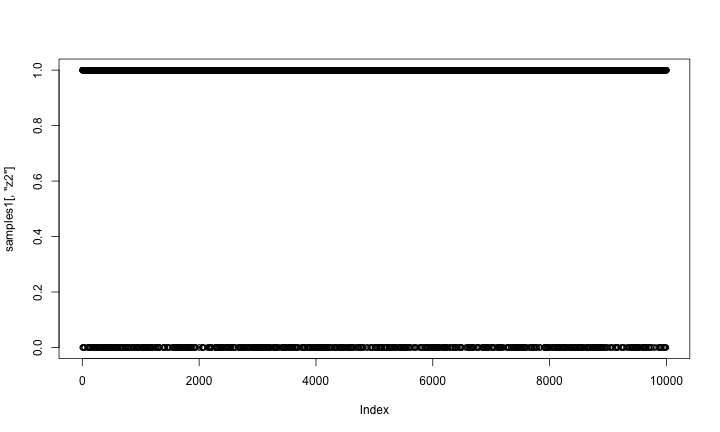
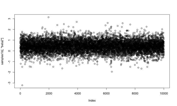
Note that the minimum overall efficiency of the AFSS sampler is approximately 28 times that of the RW_block sampler. Additionally, trace plots from the output of the AFSS sampler show that the RW_block sampler.
plot(AFSS_mcmcOutput, density = FALSE)

Tibbits, M. M, C. Groendyke, M. Haran, et al.
(2014).
“Automated factor slice sampling”.
In: Journal of Computational and Graphical Statistics 23.2, pp. 543–563.
Turek, D, P. de
Valpine, C. J. Paciorek, et al.
(2017).
“Automated parameter blocking for efficient Markov chain Monte Carlo sampling”.
In: Bayesian Analysis 12.2, pp. 465–490.
 . We define our state space model as
 ")
")
")
")
")
") is a shifted, scaled
is a shifted, scaled  -distribution with center parameter
  degrees of freedom.
  time points:


