Bayesian nonparametrics in NIMBLE: Density estimation
Overview
NIMBLE is a hierarchical modeling package that uses nearly the same language for model specification as the popular MCMC packages WinBUGS, OpenBUGS and JAGS, while making the modeling language extensible — you can add distributions and functions — and also allowing customization of the algorithms used to estimate the parameters of the model.
Recently, we added support for Markov chain Monte Carlo (MCMC) inference for Bayesian nonparametric (BNP) mixture models to NIMBLE. In particular, starting with version 0.6-11, NIMBLE provides functionality for fitting models involving Dirichlet process priors using either the Chinese Restaurant Process (CRP) or a truncated stick-breaking (SB) representation of the Dirichlet process prior.
In this post we illustrate NIMBLE’s BNP capabilities by showing how to use nonparametric mixture models with different kernels for density estimation. In a later post, we will take a parametric generalized linear mixed model and show how to switch to a nonparametric representation of the random effects that avoids the assumption of normally-distributed random effects.
For more detailed information on NIMBLE and Bayesian nonparametrics in NIMBLE, see the NIMBLE User Manual.
Basic density estimation using Dirichlet Process Mixture models
NIMBLE provides the machinery for nonparametric density estimation by means of Dirichlet process mixture (DPM) models (Ferguson, 1974; Lo, 1984; Escobar, 1994; Escobar and West, 1995). For an independent and identically distributed sample 
, \quad\quad \theta_i \mid G \sim G, \quad\quad G \mid \alpha, H \sim \mbox{DP}(\alpha, H), \quad\quad i=1,\ldots, n .")
The NIMBLE implementation of this model is flexible and allows for mixtures of arbitrary kernels, ")

To illustrate these capabilities, we consider the estimation of the probability density function of the waiting time between eruptions of the Old Faithful volcano data set available in R.
data(faithful)
The observations 
Fitting a location-scale mixture of Gaussian distributions using the CRP representation
Model specification
We first consider a location-scale Dirichlet process mixture of normal distributionss fitted to the transformed data ")
, \quad (\mu_i, \sigma^2_i) \mid G \sim G, \quad G \mid \alpha, H \sim \mbox{DP}(\alpha, H), \quad i=1,\ldots, n,")
where 
Introducing auxiliary variables 

, \quad\quad \xi \mid \alpha \sim \mbox{CRP}(\alpha), \quad\quad (\tilde{\mu}_k, \tilde{\sigma}_k^2) \mid H \sim H, \quad\quad i=1,\ldots, n ,")
where
 = \frac{\Gamma(\alpha)}{\Gamma(\alpha + n)} \alpha^{K(\xi)} \prod_k \Gamma\left(m_k(\xi)\right),")
 \le n")

")


NIMBLE’s specification of this model is given by
code <- nimbleCode({
  for(i in 1:n) {
    y[i] ~ dnorm(mu[i], var = s2[i])
    mu[i] <- muTilde[xi[i]]
    s2[i] <- s2Tilde[xi[i]]
  }
  xi[1:n] ~ dCRP(alpha, size = n)
  for(i in 1:n) {
    muTilde[i] ~ dnorm(0, var = s2Tilde[i])
    s2Tilde[i] ~ dinvgamma(2, 1)
  }
  alpha ~ dgamma(1, 1)
})
Note that in the model code the length of the parameter vectors muTilde and s2Tilde has been set to
Note also that the value of 
Running the MCMC algorithm
The following code sets up the data and constants, initializes the parameters, defines the model object, and builds and runs the MCMC algorithm. Because the specification is in terms of a Chinese restaurant process, the default sampler selected by NIMBLE is a collapsed Gibbs sampler (Neal, 2000).
set.seed(1)
# Model Data
lFaithful <- log(faithful$waiting)
standlFaithful <- (lFaithful - mean(lFaithful)) / sd(lFaithful)
data <- list(y = standlFaithful)
# Model Constants
consts <- list(n = length(standlFaithful))
# Parameter initialization
inits <- list(xi = sample(1:10, size=consts$n, replace=TRUE),
              muTilde = rnorm(consts$n, 0, sd = sqrt(10)),
              s2Tilde = rinvgamma(consts$n, 2, 1),
              alpha = 1)
# Model creation and compilation
rModel <- nimbleModel(code, data = data, inits = inits, constants = consts)
cModel <- compileNimble(rModel)
# MCMC configuration, creation, and compilation
conf <- configureMCMC(rModel, monitors = c("xi", "muTilde", "s2Tilde", "alpha"))
mcmc <- buildMCMC(conf)
cmcmc <- compileNimble(mcmc, project = rModel)
samples <- runMCMC(cmcmc, niter = 7000, nburnin = 2000, setSeed = TRUE)
## |-------------|-------------|-------------|-------------|
## |-------------------------------------------------------|
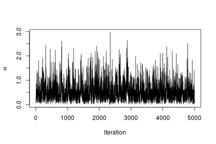
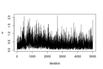
We can extract the samples from the posterior distributions of the parameters and create trace plots, histograms, and any other summary of interest. For example, for the concentration parameter
# Trace plot for the concentration parameter
ts.plot(samples[ , "alpha"], xlab = "iteration", ylab = expression(alpha))
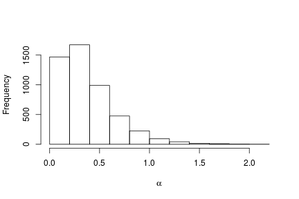
# Posterior histogram
hist(samples[ , "alpha"], xlab = expression(alpha), main = "", ylab = "Frequency")
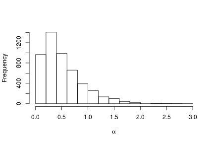
quantile(samples[ , "alpha"], c(0.5, 0.025, 0.975))
##        50%       2.5%      97.5%
## 0.42365754 0.06021512 1.52299639
Under this model, the posterior predictive distribution for a new observation 
")
# posterior samples of the concentration parameter
alphaSamples <- samples[ , "alpha"]
# posterior samples of the cluster means
muTildeSamples <- samples[ , grep('muTilde', colnames(samples))]
# posterior samples of the cluster variances
s2TildeSamples <- samples[ , grep('s2Tilde', colnames(samples))]
# posterior samples of the cluster memberships
xiSamples <- samples [ , grep('xi', colnames(samples))]

standlGrid <- seq(-2.5, 2.5, len = 200) # standardized grid on log scale

densitySamplesStandl <- matrix(0, ncol = length(standlGrid), nrow = nrow(samples))
for(i in 1:nrow(samples)){
  k <- unique(xiSamples[i, ])
  kNew <- max(k) + 1
  mk <- c()
  li <- 1
  for(l in 1:length(k)) {
    mk[li] <- sum(xiSamples[i, ] == k[li])
    li <- li + 1
  }
  alpha <- alphaSamples[i]

  muK <-  muTildeSamples[i, k]
  s2K <-  s2TildeSamples[i, k]
  muKnew <-  muTildeSamples[i, kNew]
  s2Knew <-  s2TildeSamples[i, kNew]

  densitySamplesStandl[i, ] <- sapply(standlGrid,
                function(x)(sum(mk * dnorm(x, muK, sqrt(s2K))) +
                alpha * dnorm(x, muKnew, sqrt(s2Knew)) )/(alpha+consts$n))
}

hist(data$y, freq = FALSE, xlim = c(-2.5, 2.5), ylim = c(0,0.75), main = "",
     xlab = "Waiting times on standardized log scale")
## pointwise estimate of the density for standardized log grid
lines(standlGrid, apply(densitySamplesStandl, 2, mean), lwd = 2, col = 'black')
lines(standlGrid, apply(densitySamplesStandl, 2, quantile, 0.025), lty = 2, col = 'black')
lines(standlGrid, apply(densitySamplesStandl, 2, quantile, 0.975), lty = 2, col = 'black')
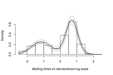
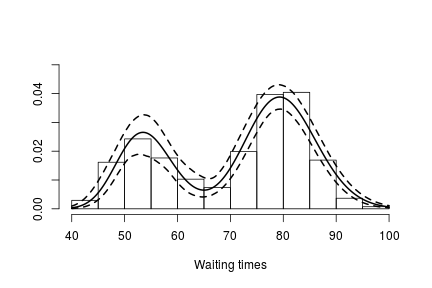
Recall, however, that this is the density estimate for the logarithm of the waiting time. To obtain the density on the original scale we need to apply the appropriate transformation to the kernel.
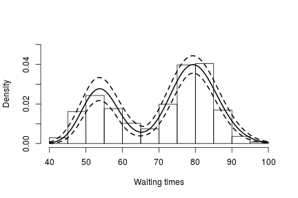
lgrid <- standlGrid*sd(lFaithful) + mean(lFaithful) # grid on log scale
densitySamplesl <- densitySamplesStandl / sd(lFaithful) # density samples for grid on log scale

hist(faithful$waiting, freq = FALSE, xlim = c(40, 100), ylim=c(0, 0.05),
     main = "", xlab = "Waiting times")
lines(exp(lgrid), apply(densitySamplesl, 2, mean)/exp(lgrid), lwd = 2, col = 'black')
lines(exp(lgrid), apply(densitySamplesl, 2, quantile, 0.025)/exp(lgrid), lty = 2,
      col = 'black')
lines(exp(lgrid), apply(densitySamplesl, 2, quantile, 0.975)/exp(lgrid), lty = 2,
      col = 'black')
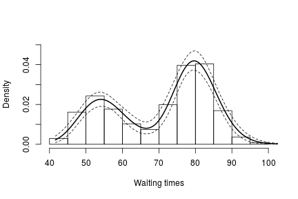
In either case, there is clear evidence that the data has two components for the waiting times.
Generating samples from the mixing distribution
While samples from the posterior distribution of linear functionals of the mixing distribution
The following code generates posterior samples from the random measure )")


outputG <- getSamplesDPmeasure(cmcmc)
## sampleDPmeasure: Approximating the random measure by a finite stick-breaking representation with and error smaller than 1e-10, leads to a truncation level of 33.
if(packageVersion('nimble') <= '0.6-12')
  samplesG <- outputG else samplesG <- outputG$samples
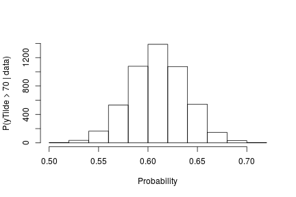
The following code computes posterior samples of ")
if(packageVersion('nimble') >= '0.6.13')
     truncG <- outputG$trunc # truncation level for G

weightIndex <- grep('weight', colnames(samplesG))
muTildeIndex <- grep('muTilde', colnames(samplesG))
s2TildeIndex <- grep('s2Tilde', colnames(samplesG))

probY70 <- rep(0, nrow(samples))  # posterior samples of P(y.tilde > 70)
for(i in seq_len(nrow(samples))) {
  probY70[i] <- sum(samplesG[i, weightIndex] *
                    pnorm(0.03557236, mean = samplesG[i, muTildeIndex],
                      sd = sqrt(samplesG[i, s2TildeIndex]), lower.tail = FALSE))
}

hist(probY70,  xlab = "Probability", ylab = "P(yTilde > 70 | data)" , main = "" )
Fitting a mixture of gamma distributions using the CRP representation
NIMBLE is not restricted to using Gaussian kernels in DPM models. In the case of the Old Faithful data, an alternative to the mixture of Gaussian kernels on the logarithmic scale that we presented in the previous section is a (scale-and-shape) mixture of Gamma distributions on the original scale of the data.
Model specification
In this case, the model takes the form
, \quad\quad \xi \mid \alpha \sim \mbox{CRP}(\alpha), \quad\quad (\tilde{\beta}_k, \tilde{\lambda}_k) \mid H \sim H ,")
where
code <- nimbleCode({
  for(i in 1:n) {
    y[i] ~ dgamma(shape = beta[i], scale = lambda[i])
    beta[i] <- betaTilde[xi[i]]
    lambda[i] <- lambdaTilde[xi[i]]
  }
  xi[1:n] ~ dCRP(alpha, size = n)
  for(i in 1:50) { # only 50 cluster parameters
    betaTilde[i] ~ dgamma(shape = 71, scale = 2)
    lambdaTilde[i] ~ dgamma(shape = 2, scale = 2)
  }
  alpha ~ dgamma(1, 1)
})
Note that in this case the vectors betaTilde and lambdaTilde have length 
Running the MCMC algorithm
The following code sets up the model data and constants, initializes the parameters, defines the model object, and builds and runs the MCMC algorithm for the mixture of Gamma distributions. Note that, when building the MCMC, a warning message about the number of cluster parameters is generated. This is because the lengths of betaTilde and lambdaTilde are smaller than
data <- list(y = faithful$waiting)
set.seed(1)
inits <- list(xi = sample(1:10, size=consts$n, replace=TRUE),
              betaTilde = rgamma(50, shape = 71, scale = 2),
              lambdaTilde = rgamma(50, shape = 2, scale = 2),
              alpha = 1)
rModel <- nimbleModel(code, data = data, inits = inits, constants = consts)
cModel <- compileNimble(rModel)
conf <- configureMCMC(rModel, monitors = c("xi", "betaTilde", "lambdaTilde", "alpha"))
mcmc <- buildMCMC(conf)
## Warning in samplerFunction(model = model, mvSaved = mvSaved, target = target, : sampler_CRP: The number of cluster parameters is less than the number of potential clusters. The MCMC is not strictly valid if ever it proposes more components than cluster parameters exist; NIMBLE will warn you if this occurs.
cmcmc <- compileNimble(mcmc, project = rModel)
samples <- runMCMC(cmcmc, niter = 7000, nburnin = 2000, setSeed = TRUE)
## |-------------|-------------|-------------|-------------|
## |-------------------------------------------------------|
In this case we use the posterior samples of the parameters to construct a trace plot and estimate the posterior distribution of
# Trace plot of the posterior samples of the concentration parameter
ts.plot(samples[ , 'alpha'], xlab = "iteration", ylab = expression(alpha))
# Histogram of the posterior samples for the concentration parameter
hist(samples[ , 'alpha'], xlab = expression(alpha), ylab = "Frequency", main = "")
Generating samples from the mixing distribution
As before, we obtain samples from the posterior distribution of
outputG <- getSamplesDPmeasure(cmcmc)
## sampleDPmeasure: Approximating the random measure by a finite stick-breaking representation with and error smaller than 1e-10, leads to a truncation level of 28.
if(packageVersion('nimble') <= '0.6-12')
  samplesG <- outputG else samplesG <- outputG$samples
We use these samples to create an estimate of the density of the data along with a pointwise 95% credible band:
if(packageVersion('nimble') >= '0.6.13')
     truncG <- outputG$trunc # truncation level for G
grid <- seq(40, 100, len = 200)

weightSamples <- samplesG[ , grep('weight', colnames(samplesG))]
betaTildeSamples <- samplesG[ , grep('betaTilde', colnames(samplesG))]
lambdaTildeSamples <- samplesG[ , grep('lambdaTilde', colnames(samplesG))]

densitySamples <- matrix(0, ncol = length(grid), nrow = nrow(samples))
for(iter in seq_len(nrow(samples))) {
  densitySamples[iter, ] <- sapply(grid, function(x)
    sum( weightSamples[iter, ] * dgamma(x, shape = betaTildeSamples[iter, ],
                scale = lambdaTildeSamples[iter, ])))
}


hist(faithful$waiting, freq = FALSE, xlim = c(40,100), ylim = c(0, .05), main = "",
   ylab = "", xlab = "Waiting times")
lines(grid, apply(densitySamples, 2, mean), lwd = 2, col = 'black')
lines(grid, apply(densitySamples, 2, quantile, 0.025), lwd = 2, lty = 2, col = 'black')
lines(grid, apply(densitySamples, 2, quantile, 0.975), lwd = 2, lty = 2, col = 'black')
Again, we see that the density of the data is bimodal, and looks very similar to the one we obtained before.
Fitting a DP mixture of Gammas using a stick-breaking representation
Model specification
An alternative representation of the Dirichlet process mixture uses the stick-breaking representation of the random distribution 
Introducing auxiliary variables, 
, \quad\quad \boldsymbol{z} \mid \boldsymbol{w} \sim \mbox{Discrete}(\boldsymbol{w}), \quad\quad ({\beta}_k^{\star}, {\lambda}_k^{\star}) \mid H \sim H ,")
where
, \quad l=2, \ldots, L-1,\quad\quad w_L=\prod_{m=1}^{L-1}(1-v_m)")
with , l=1, \ldots, L-1")
code <- nimbleCode(
  {
    for(i in 1:n) {
      y[i] ~ dgamma(shape = beta[i], scale = lambda[i])
      beta[i] <- betaStar[z[i]]
      lambda[i] <- lambdaStar[z[i]]
      z[i] ~ dcat(w[1:Trunc])
    }
    for(i in 1:(Trunc-1)) { # stick-breaking variables
      v[i] ~ dbeta(1, alpha)
    }
    w[1:Trunc] <- stick_breaking(v[1:(Trunc-1)]) # stick-breaking weights
    for(i in 1:Trunc) {
      betaStar[i] ~ dgamma(shape = 71, scale = 2)
      lambdaStar[i] ~ dgamma(shape = 2, scale = 2)
    }
    alpha ~ dgamma(1, 1)
  }
)
Note that the truncation level
Running the MCMC algorithm
The following code sets up the model data and constants, initializes the parameters, defines the model object, and builds and runs the MCMC algorithm for the mixture of Gamma distributions. When a stick-breaking representation is used, a blocked Gibbs sampler is assigned (Ishwaran, 2001; Ishwaran and James, 2002).
data <- list(y = faithful$waiting)
set.seed(1)
consts <- list(n = length(faithful$waiting), Trunc = 50)
inits <- list(betaStar = rgamma(consts$Trunc, shape = 71, scale = 2),
              lambdaStar = rgamma(consts$Trunc, shape = 2, scale = 2),
              v = rbeta(consts$Trunc-1, 1, 1),
              z = sample(1:10, size = consts$n, replace = TRUE),
              alpha = 1)

rModel <- nimbleModel(code, data = data, inits = inits, constants = consts)
cModel <- compileNimble(rModel)
conf <- configureMCMC(rModel, monitors = c("w", "betaStar", "lambdaStar", 'z', 'alpha'))
mcmc <- buildMCMC(conf)
cmcmc <- compileNimble(mcmc, project = rModel)
samples <- runMCMC(cmcmc, niter = 24000, nburnin = 4000, setSeed = TRUE)
## |-------------|-------------|-------------|-------------|
## |-------------------------------------------------------|
Using the stick-breaking approximation automatically provides an approximation, 
betaStarSamples <- samples[ , grep('betaStar', colnames(samples))]
lambdaStarSamples <- samples[ , grep('lambdaStar', colnames(samples))]
weightSamples <- samples[ , grep('w', colnames(samples))]

grid <- seq(40, 100, len = 200)

densitySamples <- matrix(0, ncol = length(grid), nrow = nrow(samples))
for(i in 1:nrow(samples)) {
  densitySamples[i, ] <- sapply(grid, function(x)
    sum(weightSamples[i, ] * dgamma(x, shape = betaStarSamples[i, ],
                                    scale = lambdaStarSamples[i, ])))
}

hist(faithful$waiting, freq = FALSE,  xlab = "Waiting times", ylim=c(0,0.05),
     main = '')
lines(grid, apply(densitySamples, 2, mean), lwd = 2, col = 'black')
lines(grid, apply(densitySamples, 2, quantile, 0.025), lwd = 2, lty = 2, col = 'black')
lines(grid, apply(densitySamples, 2, quantile, 0.975), lwd = 2, lty = 2, col = 'black')
As expected, this estimate looks identical to the one we obtained through the CRP representation of the process.
More information and future development
Please see our User Manual for more details.
We’re in the midst of improvements to the existing BNP functionality as well as adding additional Bayesian nonparametric models, such as hierarchical Dirichlet processes and Pitman-Yor processes, so please add yourself to our announcement or user support/discussion Google groups.
References
Blackwell, D. and MacQueen, J. 1973. Ferguson distributions via Polya urn schemes. The Annals of Statistics 1:353-355.
Ferguson, T.S. 1974. Prior distribution on the spaces of probability measures. Annals of Statistics 2:615-629.
Lo, A.Y. 1984. On a class of Bayesian nonparametric estimates I: Density estimates. The Annals of Statistics 12:351-357.
Escobar, M.D. 1994. Estimating normal means with a Dirichlet process prior. Journal of the American Statistical Association 89:268-277.
Escobar, M.D. and West, M. 1995. Bayesian density estimation and inference using mixtures. Journal of the American Statistical Association 90:577-588.
Ishwaran, H. and James, L.F. 2001. Gibbs sampling methods for stick-breaking priors. Journal of the American Statistical Association 96: 161-173.
Ishwaran, H. and James, L.F. 2002. Approximate Dirichlet process computing in finite normal mixtures: smoothing and prior information. Journal of Computational and Graphical Statistics 11:508-532.
Neal, R. 2000. Markov chain sampling methods for Dirichlet process mixture models. Journal of Computational and Graphical Statistics 9:249-265.
Sethuraman, J. 1994. A constructive definition of Dirichlet prior. Statistica Sinica 2: 639-650.
Chris this looks very nice.
The two ways you have of doing Dirichlet Process models look quite elegant.
The logical function you have introduced to do the stick breaking algorithm is very simple conceptually and I would guess very easy to implement. There is an example of the stick breaking approach in the BUGS examples (model Eye Tracking) however your stick_breaking function makes things muck clearer.
The Chinese Restaurant Process approach looks interesting but ii is I suspect more complex to implement dCRP. Truncating the size of the dCRP is obviously good for cutting down the run time and storage required but how do you decide how many components you need. In BUGS runtime errors are fatal but you must have test in dCRP to detect “too many” components and fail gracefully.
If the source code is available I will have a careful look through it and get back to you with any comments.
Thanks for making these two great additions to the BUGS language.
Andrew
Hi Andrew, thanks for the feedback. All our source code is at github.com/nimble-dev/nimble/packages/nimble,
with the BNP sampler code in particular at github.com/nimble-dev/nimble/packages/nimble/R/BNP_samplers.R
and the dCRP distribution at github.com/nimble-dev/nimble/packages/nimble/R/BNP_distributions.R.
We’d welcome another eye on it.
As far as how many components, if a user sets a truncation level, then if our MCMC sampling ever
tries to open too many components, we issue a warning and suggest that the user re-run the MCMC with
a lesser amount of truncation. But it does not error out.
We’re about to release our next version that should have big speed improvements in the sampling for CRP
models and will have additional improvements in the next release after that.