Posterior predictive sampling and other post-MCMC use of samples in NIMBLE
(Prepared by Chris Paciorek and Sally Paganin.)
Once one has samples from an MCMC, one often wants to do some post hoc manipulation of the samples. An important example is posterior predictive sampling, which is needed for posterior predictive checking.
With posterior predictive sampling, we need to simulate new data values, once for each posterior sample. These samples can then be compared with the actual data as a model check.
In this example, we’ll follow the posterior predictive checking done in the Gelman et al. Bayesian Data Analysis book, using Newcomb’s speed of light measurements (Section 6.3).
Posterior predictive sampling using a loop in R
Simon Newcomb made 66 measurements of the speed of light, which one might model using a normal distribution. One question discussed in Gelman et al. is whether the lowest measurements, which look like outliers, could have reasonably come from a normal distribution.
Setup
We set up the nimble model.
library(nimble, warn.conflicts = FALSE)

code <- nimbleCode({
    ## noninformative priors
    mu ~ dflat()
    sigma ~ dhalfflat()
    ## likelihood
    for(i in 1:n) {
        y[i] ~ dnorm(mu, sd = sigma)
    }
})

data <- list(y = MASS::newcomb)
inits <- list(mu = 0, sigma = 5)
constants <- list(n = length(data$y))

model <- nimbleModel(code = code, data = data, constants = constants, inits = inits)
Next we’ll create some vectors of node names that will be useful for our manipulations.
## Ensure we have the nodes needed to simulate new datasets
dataNodes <- model$getNodeNames(dataOnly = TRUE)
parentNodes <- model$getParents(dataNodes, stochOnly = TRUE)  # `getParents` is new in nimble 0.11.0
## Ensure we have both data nodes and deterministic intermediates (e.g., lifted nodes)
simNodes <- model$getDependencies(parentNodes, self = FALSE)
Now run the MCMC.
cmodel <- compileNimble(model)
mcmc <- buildMCMC(model, monitors = parentNodes)
## ===== Monitors =====
## thin = 1: mu, sigma
## ===== Samplers =====
## conjugate sampler (2)
##   - mu
##   - sigma
cmcmc <- compileNimble(mcmc, project = model)
samples <- runMCMC(cmcmc, niter = 1000, nburnin = 500)
## |-------------|-------------|-------------|-------------|
## |-------------------------------------------------------|
Posterior predictive sampling by direct variable assignment
We’ll loop over the samples and use the compiled model (uncompiled would be ok too, but slower) to simulate new datasets.
nSamp <- nrow(samples)
n <- length(data$y)
ppSamples <- matrix(0, nSamp, n)

set.seed(1)
for(i in 1:nSamp){
  cmodel[["mu"]] <- samples[i, "mu"]             ## or cmodel$mu <- samples[i, "mu"]
  cmodel[["sigma"]] <- samples[i, "sigma"]
  cmodel$simulate(simNodes, includeData = TRUE)
  ppSamples[i, ] <- cmodel[["y"]]
}
Posterior predictive sampling using values
That’s fine, but we needed to manually insert values for the different variables. For a more general solution, we can use nimble’s values function as follows.
ppSamples <- matrix(0, nrow = nSamp, ncol =
          length(model$expandNodeNames(dataNodes, returnScalarComponents = TRUE)))
postNames <- colnames(samples)

set.seed(1)
system.time({
for(i in seq_len(nSamp)) {
    values(cmodel, postNames) <- samples[i, ]  # assign 'flattened' values
    cmodel$simulate(simNodes, includeData = TRUE)
    ppSamples[i, ] <- values(cmodel, dataNodes)
}
})
##    user  system elapsed
##   4.657   0.000   4.656
Side note: For large models, it might be faster to use the variable names as the second argument to values() rather than the names of all the elements of the variables. If one chooses to do this, it’s important to check that the ordering of variables in the ‘flattened’ values in samples is the same as the ordering of variables in the second argument to values so that the first line of the for loop assigns the values from samples correctly into the model.
Doing the posterior predictive check
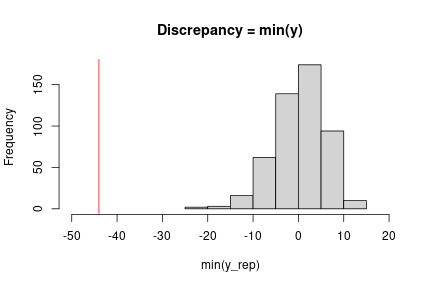
At this point, we can implement the check we want using our chosen discrepancy measure. Here a simple check uses the minimum observation.
obsMin <- min(data$y)
ppMin <- apply(ppSamples, 1, min)

# ## Check with plot in Gelman et al. (3rd edition), Figure 6.3
hist(ppMin, xlim = c(-50, 20),
    main = "Discrepancy = min(y)",
    xlab = "min(y_rep)")
abline(v = obsMin, col = 'red')
Fast posterior predictive sampling using a nimbleFunction
The approach above could be slow, even with a compiled model, because the loop is carried out in R. We could instead do all the work in a compiled nimbleFunction.
Writing the nimbleFunction
Let’s set up a nimbleFunction. In the setup code, we’ll manipulate the nodes and variables, similarly to the code above. In the run code, we’ll loop through the samples and simulate, also similarly.
Remember that all querying of the model structure needs to happen in the setup code. We also need to pass the MCMC object to the nimble function, so that we can determine at setup time the names of the variables we are copying from the posterior samples into the model.
The run code takes the actual samples as the input argument, so the nimbleFunction will work regardless of how long the MCMC was run for.
ppSamplerNF <- nimbleFunction(
          setup = function(model, mcmc) {
              dataNodes <- model$getNodeNames(dataOnly = TRUE)
              parentNodes <- model$getParents(dataNodes, stochOnly = TRUE)
              cat("Stochastic parents of data are:", paste(parentNodes, collapse = ','), ".\n")
              simNodes <- model$getDependencies(parentNodes, self = FALSE)
              vars <- mcmc$mvSamples$getVarNames()  # need ordering of variables in mvSamples / samples matrix
              cat("Using posterior samples of:", paste(vars, collapse = ','), ".\n")
              n <- length(model$expandNodeNames(dataNodes, returnScalarComponents = TRUE))
          },
          run = function(samples = double(2)) {
              nSamp <- dim(samples)[1]
              ppSamples <- matrix(nrow = nSamp, ncol = n)
              for(i in 1:nSamp) {
                    values(model, vars) <<- samples[i, ]
                    model$simulate(simNodes, includeData = TRUE)
                    ppSamples[i, ] <- values(model, dataNodes)
              }
              returnType(double(2))
              return(ppSamples)
          })
Using the nimbleFunction
We’ll create the instance of the nimbleFunction for this model and MCMC.
Then we run the compiled nimbleFunction.
## Create the sampler for this model and this MCMC.
ppSampler <- ppSamplerNF(model, mcmc)
## Stochastic parents of data are: mu,sigma .
## Using posterior samples of: mu,sigma .
cppSampler <- compileNimble(ppSampler, project = model)
## Check ordering of variables is same in 'vars' and in 'samples'.
colnames(samples)
## [1] "mu" "sigma"
identical(colnames(samples), model$expandNodeNames(mcmc$mvSamples$getVarNames()))
## [1] TRUE
set.seed(1)
system.time(ppSamples_via_nf <- cppSampler$run(samples))
##    user  system elapsed
##   0.004   0.000   0.004
identical(ppSamples, ppSamples_via_nf)
## [1] TRUE
So we get exactly the same results (note the use of set.seed to ensure this) but much faster.
Here the speed doesn’t really matter but for more samples and larger models it often will, even after accounting for the time spent to compile the nimbleFunction.
Version 0.11.1 of NIMBLE released
We’ve released the newest version of NIMBLE on CRAN and on our website. NIMBLE is a system for building and sharing analysis methods for statistical models, especially for hierarchical models and computationally-intensive methods (such as MCMC and SMC).
Version 0.11.1 is a bug fix release, fixing a bug that was introduced in Version 0.11.0 (which was released on April 17, 2021) that affected MCMC sampling in MCMCs using the “posterior_predictive_branch” sampler introduced in version 0.11.0. This sampler would be listed by name when the MCMC configuration object is created and would be assigned to any set of multiple nodes that (as a group of nodes) have no data dependencies and are therefore sampled as a group from their predictive distributions.
For those currently using version 0.11.0, please update your version of NIMBLE. For users currently using other versions, this release won’t directly affect you, but we generally encourage you to update as we release new versions.
Version 0.11.0 of NIMBLE released
- added the ‘posterior_predictive_branch’ MCMC sampler, which samples jointly from the predictive distribution of networks of entirely non-data nodes, to improve MCMC mixing,
- added a model method to find parent nodes, called getParents(), analogous to getDependencies(),
- improved efficiency of conjugate samplers,
- allowed use of the elliptical slice sampler for univariate nodes, which can be useful for posteriors with multiple modes,
- allowed model definition using if-then-else without an else clause, and
- fixed a bug giving incorrect node names and potentially affecting algorithm behavior for models with more than 100,000 elements in a vector node or any dimension of a multi-dimensional node.
Please see the release notes on our website for more details.
Bayesian Nonparametric Models in NIMBLE: General Multivariate Models
(Prepared by Claudia Wehrhahn)
Overview
NIMBLE is a hierarchical modeling package that uses nearly the same language for model specification as the popular MCMC packages WinBUGS, OpenBUGS and JAGS, while making the modeling language extensible — you can add distributions and functions — and also allowing customization of the algorithms used to estimate the parameters of the model.
NIMBLE supports Markov chain Monte Carlo (MCMC) inference for Bayesian nonparametric (BNP) mixture models. Specifically, NIMBLE provides functionality for fitting models involving Dirichlet process priors using either the Chinese Restaurant Process (CRP) or a truncated stick-breaking (SB) representation.
In version 0.10.1, we’ve extended NIMBLE to be able to handle more general multivariate models when using the CRP prior. In particular, one can now easily use the CRP prior when multiple observations (or multiple latent variables) are being jointly clustered. For example, in a longitudinal study, one may want to cluster at the individual level, i.e., to jointly cluster all of the observations for each of the individuals in the study. (Formerly this was only possible in NIMBLE by specifying the observations for each individual as coming from a single multivariate distribution.)
This allows one to specify a multivariate mixture kernel as the product of univariate ones. This is particularly useful when working with discrete data. In general, multivariate extensions of well-known univariate discrete distributions, such as the Bernoulli, Poisson and Gamma, are not straightforward. For example, for multivariate count data, a multivariate Poisson distribution might appear to be a good fit, yet its definition is not trivial, inference is cumbersome, and the model lacks flexibility to deal with overdispersion. See Inouye et al. (2017) for a review on multivariate distributions for count data based on the Poisson distribution.
In this post, we illustrate NIMBLE’s new extended BNP capabilities by modelling multivariate discrete data. Specifically, we show how to model multivariate count data from a longitudinal study under a nonparametric framework. The modeling approach is simple and introduces correlation in the measurements within subjects.
For more detailed information on NIMBLE and Bayesian nonparametrics in NIMBLE, see the User Manual.
BNP analysis of epileptic seizure count data
We illustrate the use of nonparametric multivariate mixture models for modeling counts of epileptic seizures from a longitudinal study of the drug progabide as an adjuvant antiepileptic chemotherapy. The data, originally reported in Leppik et al. (1985), arise from a clinical trial of 59 people with epilepsy. At four clinic visits, subjects reported the number of seizures occurring over successive two-week periods. Additional data include the baseline seizure count and the age of the patient. Patients were randomized to receive either progabide or a placebo, in addition to standard chemotherapy.
load(url("https://r-nimble.org/nimbleExamples/seizures.Rda"))
names(seizures)
## [1] "id" "seize" "visit" "trt" "age"
head(seizures)
##    id seize visit trt age
## 1 101    76     0   1  18
## 2 101    11     1   1  18
## 3 101    14     2   1  18
## 4 101     9     3   1  18
## 5 101     8     4   1  18
## 6 102    38     0   1  32
Model formulation
We model the joint distribution of the baseline number of seizures and the counts from each of the two-week periods as a Dirichlet Process mixture (DPM) of products of Poisson distributions. Let ")


where ")

, \quad\quad \boldsymbol{\lambda}_{i} \mid G \sim G, \quad\quad G \sim DP(\alpha, H),")
Our specification uses a product of Poisson distributions as the kernel in the DPM which, at first sight, would suggest independence of the repeated seizure count measurements. However, because we are mixing over the parameters, this specification in fact induces dependence within subjects, with the strength of the dependence being inferred from the data. In order to specify the model in NIMBLE, first we translate the information in seize into a matrix and then we write the NIMBLE code.
We specify this model in NIMBLE with the following code in R. The vector xi contains the latent cluster IDs, one for each patient.
n <- 59
J <- 5
data <- list(y = matrix(seizures$seize, ncol = J, nrow = n, byrow = TRUE))
constants <- list(n = n, J = J)

code <- nimbleCode({
  for(i in 1:n) {
    for(j in 1:J) {
      y[i, j] ~ dpois(lambda[xi[i], j])
    }
  }
  for(i in 1:n) {
    for(j in 1:J) {
      lambda[i, j] ~ dgamma(shape = 1, rate = 0.1)
    }
  }
  xi[1:n] ~ dCRP(conc = alpha, size = n)
  alpha ~ dgamma(shape = 1, rate = 1)
})
Running the MCMC
The following code sets up the data and constants, initializes the parameters, defines the model object, and builds and runs the MCMC algorithm. For speed, the MCMC runs using compiled C++ code, hence the calls to compileNimble to create compiled versions of the model and the MCMC algorithm.
Because the specification is in terms of a Chinese restaurant process, the default sampler selected by NIMBLE is a collapsed Gibbs sampler. More specifically, because the baseline distribution
set.seed(1)
inits <- list(xi = 1:n, alpha = 1,
             lambda = matrix(rgamma(J*n, shape = 1, rate = 0.1), ncol = J, nrow = n))
model <- nimbleModel(code, data=data, inits = inits, constants = constants, dimensions = list(lambda = c(n, J)))
cmodel <- compileNimble(model)
conf <- configureMCMC(model, monitors = c('xi','lambda', 'alpha'), print = TRUE)
## ===== Monitors =====
## thin = 1: xi, lambda, alpha
## ===== Samplers =====
## CRP_concentration sampler (1)
##   - alpha
## CRP_cluster_wrapper sampler (295)
##   - lambda[]  (295 elements)
## CRP sampler (1)
##   - xi[1:59]
mcmc <- buildMCMC(conf)
cmcmc <- compileNimble(mcmc, project = model)
samples <- runMCMC(cmcmc, niter=55000, nburnin = 5000, thin=10)
## |-------------|-------------|-------------|-------------|
## |-------------------------------------------------------|
We can extract posterior samples for some parameters of interest. The following are trace plots of the posterior samples for the concentration parameter, 
xiSamples <- samples[, grep('xi', colnames(samples))]    # samples of cluster IDs
nGroups <- apply(xiSamples, 1, function(x)  length(unique(x)))
concSamples <- samples[, grep('alpha', colnames(samples))]

par(mfrow=c(1, 2))
ts.plot(concSamples, xlab = "Iteration", ylab = expression(alpha), main = expression(paste('Traceplot for ', alpha)))
ts.plot(nGroups,  xlab = "Iteration", ylab = "Number of components", main = "Number of clusters")

Assessing the posterior
We can compute the posterior predictive distribution for a new observation 
")

")
# samples from the random measure
samplesG <- getSamplesDPmeasure(cmcmc)
niter <- length(samplesG)
weightsIndex <- grep('weights', colnames(samplesG[[1]]))
lambdaIndex <- grep('lambda', colnames(samplesG[[1]]))
ygrid <- 0:45

# function used to compute bivariate posterior predictive
bivariateFun <- nimbleFunction(
  run = function(w = double(1),
               lambda1 = double(1),
               lambda5 = double(1),
               ytilde = double(1)) {
    returnType(double(2))

    ngrid <- length(ytilde)
    out <- matrix(0, ncol = ngrid, nrow = ngrid)

    for(i in 1:ngrid) {
      for(j in 1:ngrid) {
        out[i, j] <- sum(w * dpois(ytilde[i], lambda1) * dpois(ytilde[j], lambda5))
      }
    }

    return(out)
  }
)
cbivariateFun <- compileNimble(bivariateFun)
# computing bivariate posterior predictive of seizure counts are baseline and fourth visit
bivariate <- matrix(0, ncol = length(ygrid), nrow = length(ygrid))
for(iter in 1:niter) {
  weights <- samplesG[[iter]][, weightsIndex] # posterior weights
  lambdaBaseline <- samplesG[[iter]][, lambdaIndex[1]] # posterior rate of baseline
  lambdaVisit4 <- samplesG[[iter]][, lambdaIndex[5]] # posterior rate at fourth visit
  bivariate <- bivariate + cbivariateFun(weights, lambdaBaseline, lambdaVisit4, ygrid)
}
bivariate <- bivariate / niter
The following code creates a heatmap of the posterior predictive bivariate distribution of the number of seizures at baseline and at the fourth hospital visit, showing that there is a positive correlation between these two measurements.
collist <- colorRampPalette(c('white', 'grey', 'black'))
image.plot(ygrid, ygrid, bivariate, col = collist(6),
           xlab = 'Baseline', ylab = '4th visit', ylim = c(0, 15), axes = TRUE)

In order to describe the uncertainty in the posterior clustering structure of the individuals in the study, we present a heat map of the posterior probability of two subjects belonging to the same cluster. To do this, first we compute the posterior pairwise clustering matrix that describes the probability of two individuals belonging to the same cluster, then we reorder the observations and finally plot the associated heatmap.
pairMatrix <- apply(xiSamples, 2, function(focal) {
                                   colSums(focal == xiSamples)
                                  })
pairMatrix <- pairMatrix / niter


newOrder <- c(1, 35, 13, 16, 32, 33,  2, 29, 39, 26, 28, 52, 17, 15, 23,  8, 31,
              38,  9, 46, 45, 11, 49, 44, 50, 41, 54, 21,  3, 40, 47, 48, 12,
              6, 14,  7, 18, 22, 30, 55, 19, 34, 56, 57,  4,  5, 58, 10, 43, 25,
              59, 20, 27, 24, 36, 37, 42, 51, 53)

reordered_pairMatrix <- pairMatrix[newOrder, newOrder]
image.plot(1:n, 1:n, reordered_pairMatrix , col = collist(6),
           xlab = 'Patient', ylab = 'Patient',  axes = TRUE)
axis(1, at = 1:n, labels = FALSE, tck = -.02)
axis(2, at = 1:n, labels = FALSE, tck = -.02)
axis(3, at = 1:n, tck = 0, labels = FALSE)
axis(4, at = 1:n, tck = 0, labels = FALSE)

References
Inouye, D.I., E. Yang, G.I. Allen, and P. Ravikumar. 2017. A Review of Multivariate Distributions for Count Data Derived from the Poisson Distribution. Wiley Interdisciplinary Reviews: Computational Statistics 9: e1398.
Leppik, I., F. Dreifuss, T. Bowman, N. Santilli, M. Jacobs, C. Crosby, J. Cloyd, et al. 1985. A Double-Blind Crossover Evaluation of Progabide in Partial Seizures: 3: 15 Pm8. Neurology 35.
Neal, R. 2000. Markov chain sampling methods for Dirichlet process mixture models. Journal of Computational and Graphical Statistics 9: 249–65.
NIMBLE virtual short course, May 26-28
We’ll be holding a virtual training workshop on NIMBLE, May 26-28, from 8 am to 1 pm US Pacific (California) time each day. NIMBLE is a system for building and sharing analysis methods for statistical models, especially for hierarchical models and computationally-intensive methods (such as MCMC and SMC).
The workshop will roughly follow the material covered in our June 2020 virtual training, in particular:
- the basic concepts and workflows for using NIMBLE and converting BUGS or JAGS models to work in NIMBLE.
- overview of different MCMC sampling strategies and how to use them in NIMBLE.
- writing new distributions and functions for more flexible modeling and more efficient computation.
- tips and tricks for improving computational efficiency.
- using advanced model components, including Bayesian non-parametric distributions (based on Dirichlet process priors), conditional auto-regressive (CAR) models for spatially correlated random fields, and reversible jump samplers for variable selection.
- an introduction to programming new algorithms in NIMBLE.
- calling R and compiled C++ code from compiled NIMBLE models or functions.
If participant interests vary sufficiently, the third session will be split into two tracks. One of these will likely focus on ecological models. The other will be chosen based on attendee interest from topics such as (a) advanced NIMBLE programming including writing new MCMC samplers, (b) advanced spatial or Bayesian non-parametric modeling, or (c) non-MCMC algorithms in NIMBLE, such as sequential Monte Carlo.
If you are interested in attending, please pre-register at https://forms.gle/6AtNgfdUdvhni32Q6. This will hold a spot for you and allow us to learn about your specific interests. No payment is necessary to pre-register. Fees to finalize registration will be $100 (regular) or $50 (student). We will offer a process for students to request a fee waiver.
The workshop will assume attendees have a basic understanding of hierarchical/Bayesian models and MCMC, the BUGS (or JAGS) model language, and some familiarity with R.
NIMBLE is hiring a programmer
The NIMBLE development team is hiring for a one-year programmer position. We are looking for someone with R and C++ experience. There is also a possibility of a part-time position. The deadline for full consideration is February 12. Application information is here: https://aprecruit.berkeley.edu/JPF02822.
Version 0.10.1 of NIMBLE released
– In particular, it fixes a bug in retrieving parameter values from distributions that was introduced in version 0.10.0. The bug can cause incorrect behavior of conjugate MCMC samplers under certain model structures (such as particular state-space models), so we strongly encourage users to upgrade to 0.10.1.
– In addition, version 0.10.1 restricts use of WAIC to the conditional version of WAIC (conditioning on all parameters directly involved in the likelihood). Previous versions of nimble gave incorrect results when not conditioning on all parameters directly involved in the likelihood (i.e., when not monitoring all such parameters). In a future version of nimble we plan to make a number of improvements to WAIC, including allowing use of marginal versions of WAIC, where the WAIC calculation integrates over random effects.
NIMBLE’s sequential Monte Carlo (SMC) algorithms are now in the nimbleSMC package
We’ve moved NIMBLE’s various sequential Monte Carlo (SMC) algorithms (bootstrap particle filter, auxiliary particle filter, ensemble Kalman filter, iterated filter2, and particle MCMC algorithms) to the new nimbleSMC package. So if you want to use any of these methods as of nimble version 0.10.0, please make sure to install the nimbleSMC package. Any existing code you have that uses any SMC functionality should continue to work as is.
Version 0.10.0 of NIMBLE released
We’ve released the newest version of NIMBLE on CRAN and on our website. NIMBLE is a system for building and sharing analysis methods for statistical models, especially for hierarchical models and computationally-intensive methods (such as MCMC and SMC).
- greatly extended NIMBLE’s Chinese Restaurant Process (CRP)-based Bayesian nonparametrics functionality by allowing multiple observations to be grouped together;
- fixed a bug giving incorrect results in our cross-validation function, runCrossValidate();
- moved NIMBLE’s sequential Monte Carlo (SMC, aka particle filtering) methods into the nimbleSMC package; and
- improved the efficiency of model and MCMC building and compilation.
Please see the release notes on our website for more details.
New NIMBLE cheatsheat available