Prepared by Sally Paganin.

Reversible Jump MCMC Overview

Reversible Jump MCMC (RJMCMC) is a general framework for MCMC simulation in which the dimension of the parameter space (i.e., the number of parameters) can vary between iterations of the Markov chain. It can be viewed as an extension of the Metropolis-Hastings algorithm onto more general state spaces. A common use case for RJMCMC is for variable selection in regression-style problems, where the dimension of the parameter space varies as variables are included or excluded from the regression specification.

Recently we added an RJMCMC sampler for variable selection to NIMBLE, using a univariate normal distribution as proposal distribution. There are two ways to use RJMCMC variable selection in your model. If you know the prior probability for inclusion of a variable in the model, you can use that directly in the RJMCMC without modifying your model. If you need the prior probability for inclusion in the model to be a model node itself, such as if it will have a prior and be estimated, you will need to write the model with indicator variables. In this post we will illustrate the basic usage of NIMBLE RJMCMC in both situations.

More information can be found in the NIMBLE User Manual and via help(configureRJ).

Linear regression example

In the following we consider a linear regression example in which we have 15 explanatory variables, and five of those are real effects while the others have no effect. First we simulate some data.

N <- 100
p <- 15
set.seed(1)
X <- matrix(rnorm(N*p), nrow = N, ncol = p)
true_betas <- c(c(0.1, 0.2, 0.3, 0.4, 0.5),
                rep(0, 10))

y <- rnorm(N, X%*%true_betas, sd = 1)

summary(lm(y ~ X))

## 
## Call:
## lm(formula = y ~ X)
## 
## Residuals:
##      Min       1Q   Median       3Q      Max 
## -2.64569 -0.50496  0.01613  0.59480  1.97766 
## 
## Coefficients:
##             Estimate Std. Error t value Pr(>|t|)    
## (Intercept) -0.04190    0.11511  -0.364   0.7168    
## X1           0.06574    0.12113   0.543   0.5888    
## X2           0.21162    0.11469   1.845   0.0686 .  
## X3           0.16606    0.10823   1.534   0.1287    
## X4           0.66582    0.11376   5.853 9.06e-08 ***
## X5           0.51343    0.09351   5.490 4.18e-07 ***
## X6           0.01506    0.11399   0.132   0.8952    
## X7          -0.12203    0.10127  -1.205   0.2316    
## X8           0.18177    0.10168   1.788   0.0774 .  
## X9          -0.09645    0.10617  -0.908   0.3663    
## X10          0.15986    0.11294   1.416   0.1606    
## X11          0.03806    0.10530   0.361   0.7186    
## X12          0.05354    0.10834   0.494   0.6225    
## X13         -0.02510    0.10516  -0.239   0.8119    
## X14         -0.07184    0.12842  -0.559   0.5774    
## X15         -0.04327    0.11236  -0.385   0.7011    
## ---
## Signif. codes:  0 '***' 0.001 '**' 0.01 '*' 0.05 '.' 0.1 ' ' 1
## 
## Residual standard error: 1.035 on 84 degrees of freedom
## Multiple R-squared:  0.5337,	Adjusted R-squared:  0.4505 
## F-statistic:  6.41 on 15 and 84 DF,  p-value: 7.726e-09

Reversible jump with indicator variables

Next we set up the model. In this case we explicitly include indicator variables that include or exclude the corresponding predictor variable. For this example we assume the indicator variables are exchangeable and we include the inclusion probability in the inference.

lmIndicatorCode <- nimbleCode({
  sigma ~ dunif(0, 20)  ## uniform prior per Gelman (2006)
  psi ~ dunif(0,1)    ## prior on inclusion probability

  for(i in 1:numVars) {
    z[i] ~ dbern(psi) ## indicator variable for each coefficient
    beta[i] ~ dnorm(0, sd = 100)
    zbeta[i] <- z[i] * beta[i]  ## indicator * beta
  }
  for(i in 1:N) {
    pred.y[i] <- inprod(X[i, 1:numVars], zbeta[1:numVars])
    y[i] ~ dnorm(pred.y[i], sd = sigma)
  }
})

## Set up the model.
lmIndicatorConstants <- list(N = 100, numVars = 15)
lmIndicatorInits <- list(sigma = 1, psi = 0.5,
                         beta = rnorm(lmIndicatorConstants$numVars),
                         z = sample(0:1, lmIndicatorConstants$numVars, 0.5))

lmIndicatorData  <- list(y = y, X = X)
lmIndicatorModel <- nimbleModel(code = lmIndicatorCode, constants = lmIndicatorConstants,
                                inits = lmIndicatorInits, data = lmIndicatorData)

## defining model...

## building model...

## setting data and initial values...

## running calculate on model (any error reports that follow may simply reflect missing values in model variables) ... 
## checking model sizes and dimensions...
## model building finished.

The above model code can potentially be used to set up variable selection in NIMBLE without using RJMCMC, since the indicator variables can turn the regression parameters off and on. However, in that case the MCMC sampling can be inefficient because a given regression parameter can wander widely in the parameter space when the corresponding variable is not in the model. This can make it difficult for the variable to be put back into the model, unless the prior for that variable is (perhaps artificially) made somewhat informative. Configuring RJMCMC sampling via our NIMBLE function configureRJ results in the MCMC not sampling the regression coefficients for variables for iterations where the variables are not in the model.

Configuring RJMCMC

The RJMCMC sampler can be added to the MCMC configuration by calling the function configureRJ(). In the example considered we introduced z as indicator variables associated with the regression coefficients beta. We can pass these, respectively, to configureRJ using the arguments indicatorNodes and targetNodes. The control arguments allow one to specify the mean and the scale of the normal proposal distribution used when proposing to put a coefficient back into the model.

lmIndicatorConf <- configureMCMC(lmIndicatorModel)
lmIndicatorConf$addMonitors('z')

## thin = 1: sigma, psi, beta, z

configureRJ(lmIndicatorConf,
            targetNodes = 'beta',
            indicatorNodes = 'z',
            control = list(mean = 0, scale = .2))

Checking the assigned samplers we see that the indicator variables are each assigned an RJ_indicator sampler whose targetNode is the corresponding coefficient, while the beta parameters have a RJ_toggled sampler. The latter sampler is a modified version of the original sampler to the targetNode that is invoked only when the variable is currently in the model.

## Check the assigned samplers
lmIndicatorConf$printSamplers(c("z[1]", "beta[1]"))

## [3] RJ_indicator sampler: z[1],  mean: 0,  scale: 0.2,  targetNode: beta[1]
## [4] RJ_toggled sampler: beta[1],  samplerType: conjugate_dnorm_dnorm

Build and run the RJMCMC

mcmcIndicatorRJ <- buildMCMC(lmIndicatorConf)

cIndicatorModel <- compileNimble(lmIndicatorModel)

## compiling... this may take a minute. Use 'showCompilerOutput = TRUE' to see C++ compilation details.

## compilation finished.

CMCMCIndicatorRJ <- compileNimble(mcmcIndicatorRJ, project = lmIndicatorModel)

## compiling... this may take a minute. Use 'showCompilerOutput = TRUE' to see C++ compilation details.
## compilation finished.

set.seed(1)
system.time(samplesIndicator <- runMCMC(CMCMCIndicatorRJ, niter = 10000, nburnin = 1000))

## running chain 1...

## |-------------|-------------|-------------|-------------|
## |-------------------------------------------------------|

##    user  system elapsed 
##   2.749   0.004   2.753

Looking at the results

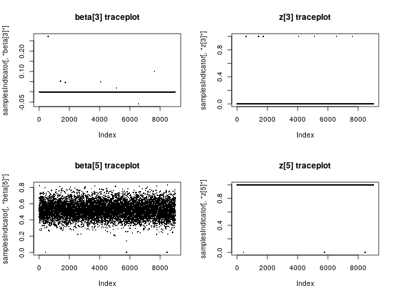
We can look at the sampled values of the indicator and corresponding coefficient for some of the variables.

par(mfrow = c(2, 2))
plot(samplesIndicator[,'beta[3]'], pch = 16, cex = 0.4, main = "beta[3] traceplot")
plot(samplesIndicator[,'z[3]'], pch = 16, cex = 0.4, main = "z[3] traceplot")
plot(samplesIndicator[,'beta[5]'], pch = 16, cex = 0.4, main = "beta[5] traceplot")
plot(samplesIndicator[,'z[5]'], pch = 16, cex = 0.4, main = "z[5] traceplot")

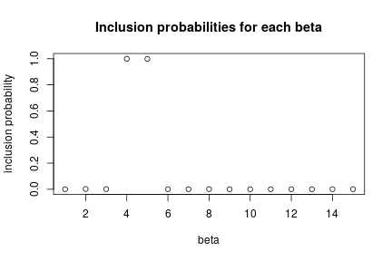
Individual inclusion probabilities

Now let’s look at the inference on the variable selection problem. We see that the fourth and fifth predictors are almost always included (these are the ones with the largest true coefficient values), while the others, including some variables that are truly associated with the outcome but have smaller true coefficient values, are almost never included.

par(mfrow = c(1, 1))
zCols <- grep("z\\[", colnames(samplesIndicator))
posterior_inclusion_prob <- colMeans(samplesIndicator[, zCols])
plot(1:length(true_betas), posterior_inclusion_prob,
        xlab = "beta", ylab = "inclusion probability",
        main = "Inclusion probabilities for each beta")

Reversible jump without indicator variables

If we assume that the inclusion probabilities for the coefficients are known, we can use the RJMCMC with model code written without indicator variables.

lmNoIndicatorCode <- nimbleCode({
  sigma ~ dunif(0, 20)

  for(i in 1:numVars) {
    beta[i] ~ dnorm(0, sd = 100)
  }
  for(i in 1:N) {
    pred.y[i] <- inprod(X[i, 1:numVars], beta[1:numVars])
    y[i] ~ dnorm(pred.y[i], sd = sigma)
  }
})

## Define model constants, inits and data
lmNoIndicatorConstants <- list(N = 100, numVars = 15)
lmNoIndicatorInits <- list(sigma = 1,
                           beta = rnorm(lmNoIndicatorConstants$numVars))
lmNoIndicatorData  <- list(y = y, X = X)

lmNoIndicatorModel <- nimbleModel(code = lmNoIndicatorCode,
                                  constants = lmNoIndicatorConstants,
                                  inits = lmNoIndicatorInits,
                                  data = lmNoIndicatorData)

## defining model...

## building model...

## setting data and initial values...

## running calculate on model (any error reports that follow may simply reflect missing values in model variables) ... 
## checking model sizes and dimensions...
## model building finished.

Configuring RJMCMC with no indicator variables

Again, the RJMCMC sampler can be added to the MCMC configuration by calling the function configureRJ() for nodes specified in targetNodes, but since there are no indicator variables we need to provide the prior inclusion probabilities. We use the priorProb argument, and we can provide either a vector of values or a common value.

lmNoIndicatorConf <- configureMCMC(lmNoIndicatorModel)
configureRJ(lmNoIndicatorConf,
            targetNodes = 'beta',
            priorProb = 0.5,
            control = list(mean = 0, scale = .2))

Since there are no indicator variables in this case, a RJ_fixed_prior sampler is assigned directly to each of coefficents along with the RJ_toggled sampler, which still uses the default sampler for the node, but only if the corresponding variable is in the model at a given iteration. In addition in this case one can set the coefficient to a value different from zero via the fixedValue argument in the control list.

## Check the assigned samplers
lmNoIndicatorConf$printSamplers(c("beta[1]"))

## [2] RJ_fixed_prior sampler: beta[1],  priorProb: 0.5,  mean: 0,  scale: 0.2,  fixedValue: 0
## [3] RJ_toggled sampler: beta[1],  samplerType: conjugate_dnorm_dnorm,  fixedValue: 0

Build and run the RJMCMC

mcmcNoIndicatorRJ <- buildMCMC(lmNoIndicatorConf)

cNoIndicatorModel <- compileNimble(lmNoIndicatorModel)

## compiling... this may take a minute. Use 'showCompilerOutput = TRUE' to see C++ compilation details.

## compilation finished.

CMCMCNoIndicatorRJ <- compileNimble(mcmcNoIndicatorRJ, project = lmNoIndicatorModel)

## compiling... this may take a minute. Use 'showCompilerOutput = TRUE' to see C++ compilation details.
## compilation finished.

set.seed(100)
system.time(samplesNoIndicator <- runMCMC(CMCMCNoIndicatorRJ, niter = 10000, nburnin = 1000))

## running chain 1...

## |-------------|-------------|-------------|-------------|
## |-------------------------------------------------------|

##    user  system elapsed 
##   3.014   0.004   3.050

Looking at the results

In this case we just look at one of the model coefficients.

plot(samplesNoIndicator[,'beta[1]'], pch = 16, cex = 0.4, main = "beta[1] traceplot")

Individual inclusion proportion

We can calculate the proportion of times each coefficient is included in the model.

betaCols <- grep("beta\\[", colnames(samplesNoIndicator))
posterior_inclusion_proportions <- colMeans(apply(samplesNoIndicator[, betaCols],
                                                  2, function(x) x != 0))
posterior_inclusion_proportions

##      beta[1]      beta[2]      beta[3]      beta[4]      beta[5] 
## 0.0017777778 0.0097777778 0.0017777778 1.0000000000 0.9996666667 
##      beta[6]      beta[7]      beta[8]      beta[9]     beta[10] 
## 0.0015555556 0.0015555556 0.0031111111 0.0018888889 0.0028888889 
##     beta[11]     beta[12]     beta[13]     beta[14]     beta[15] 
## 0.0006666667 0.0015555556 0.0007777778 0.0024444444 0.0007777778

We’ve posted a variety of new code examples for NIMBLE at https://r-nimble.org/examples.

These include some introductory code for getting started with NIMBLE, as well as examples of setting up specific kinds of models such as GLMMs, spatial models, item-response theory models, and a variety of models widely used in ecology. We also have examples of doing variable selection via reversible jump MCMC, using MCEM, and writing new distributions for use with NIMBLE.

And if you have examples that you think might be useful to make available to others, please get in touch with us.