Version 0.8.0 of NIMBLE released

Posted on June 7, 2019June 7, 2019 by Chris Paciorek

We’ve released the newest version of NIMBLE on CRAN and on our website. NIMBLE is a system for building and sharing analysis methods for statistical models, especially for hierarchical models and computationally-intensive methods (such as MCMC and SMC). Version 0.8.0 provides some new features, speed improvements, and a variety of bug fixes and better error/warning messages.

New features include:

a reversible jump MCMC sampler for variable selection via configureRJ();
greatly improved speed of MCMC sampling for Bayesian nonparametric models with a dCRP distribution by not sampling parameters for empty clusters;
experimental faster MCMC configuration, available by setting nimbleOptions(oldConjugacyChecking = FALSE) and nimbleOptions(useNewConfigureMCMC = TRUE);
and improved warning and error messages for MCEM and slice sampling.

Please see the release notes on our website for more details.

Version 0.7.1 of NIMBLE released

Posted on March 15, 2019March 15, 2019 by Chris Paciorek

Version 0.7.1 is primarily a maintenance release with a couple important bug fixes and a few additional features. Users with large models and users of the dCRP Bayesian nonparametric distribution are strongly encouraged to update to this version to pick up the bug fixes related to these uses.

New features include:

recognition of normal-normal conjugacy in additional multivariate regression settings;
handling of six-dimensional arrays in models.

Please see the release notes on our website for more details.

Version 0.7.0 of NIMBLE released

Posted on February 5, 2019February 5, 2019 by Chris Paciorek

We’ve released the newest version of NIMBLE on CRAN and on our website. NIMBLE is a system for building and sharing analysis methods for statistical models, especially for hierarchical models and computationally-intensive methods (such as MCMC and SMC). Version 0.7.0 provides a variety of new features, as well as various bug fixes.

New features include:

greatly improved efficiency of sampling for Bayesian nonparametric (BNP) mixture models that use the dCRP (Chinese Restaurant process) distribution;
addition of the double exponential (Laplace) distribution for use in models and nimbleFunctions;
a new “RW_wishart” MCMC sampler, for sampling non-conjugate Wishart and inverse-Wishart nodes;
handling of the normal-inverse gamma conjugacy for BNP mixture models using the dCRP distribution;
enhanced functionality of the getSamplesDPmeasure function for posterior sampling from BNP random measures with Dirichlet process priors.
handling of five-dimensional arrays in models;
enhanced warning messages; and
an HTML version of the NIMBLE manual.

Please see the NEWS file in the installed package for more details.

Bayesian Nonparametric Models in NIMBLE, Part 2: Nonparametric Random Effects

Posted on December 6, 2018December 6, 2018 by Chris Paciorek

Bayesian nonparametrics in NIMBLE: Nonparametric random effects

Overview

NIMBLE is a hierarchical modeling package that uses nearly the same language for model specification as the popular MCMC packages WinBUGS, OpenBUGS and JAGS, while making the modeling language extensible — you can add distributions and functions — and also allowing customization of the algorithms used to estimate the parameters of the model.

Recently, we added support for Markov chain Monte Carlo (MCMC) inference for Bayesian nonparametric (BNP) mixture models to NIMBLE. In particular, starting with version 0.6-11, NIMBLE provides functionality for fitting models involving Dirichlet process priors using either the Chinese Restaurant Process (CRP) or a truncated stick-breaking (SB) representation of the Dirichlet process prior.

We will illustrate NIMBLE’s BNP capabilities using two examples. In a previous post, we showed how to use nonparametric mixture models with different kernels for density estimation. In this post, we will take a parametric generalized linear mixed model and show how to switch to a nonparametric representation of the random effects that avoids the assumption of normally-distributed random effects.

For more detailed information on NIMBLE and Bayesian nonparametrics in NIMBLE, see the NIMBLE User Manual.

Parametric meta analysis of Avandia myocardial infarctions (MIs)

We will illustrate the use of nonparametric mixture models for modeling random effects distributions in the context of a meta-analysis of the side effects of a formerly very popular drug for diabetes called Avandia. The data we analyze played a role in raising serious questions about the safety of this drug. The question is whether Avandia use increases the risk of myocardial infarction (heart attack). There are 48 studies (the 49th study in the data file is different in some ways and excluded here), each with treatment and control arms.

dat <- read.csv('https://rawgit.com/nimble-dev/nimble-demos/master/intro_bnp/avandia.csv')
head(dat)

##   trial nAvandia avandiaMI nControl controlMI
## 1     1      357         2      176         0
## 2     2      391         2      207         1
## 3     3      774         1      185         1
## 4     4      213         0      109         1
## 5     5      232         1      116         0
## 6     6       43         0       47         1

dat <- dat[-49, ]

Model formulation

We begin with a standard generalized linear mixed model (GLMM)-based meta analysis. The vectors $n$ and $x$ contain the total number of patients in the control and the number of patients suffering from myocardial infarctions in the control group of each study, respectively. Similarly, the vectors $m$ and $y$ contain similar information for patients receiving the drug Avandia. The model takes the form

$x_{i} \mid \theta, \gamma_i \sim \mbox{Bin} \left(n_i, \frac{\exp\left\{ \gamma_i \right\}}{1 + \exp\left\{ \gamma_i \right\}} \right) , \quad\quad y_{i} \mid \theta, \gamma_i \sim \mbox{Bin} \left(m_i, \frac{\exp\left\{ \theta + \gamma_i \right\}}{1 + \exp\left\{ \theta + \gamma_i \right\}} \right)$

where the random effects, $\gamma_i$ , follow a common normal distribution, $\gamma_i \sim \mbox{N}(0, \tau^2)$ , and the $\theta$ and $\tau^2$ are given reasonably non-informative priors. The parameter $\theta$ quantifies the difference in risk between the control and treatment arms, while the $\gamma_i$ quantify study-specific variation.

This model can be specified in NIMBLE using the following code:

x <- dat$controlMI
n <- dat$nControl
y <- dat$avandiaMI
m <- dat$nAvandia

nStudies <- nrow(dat)
data <- list(x = x, y = y)
constants = list(n = n, m = m, nStudies = nStudies)

codeParam <- nimbleCode({
    for(i in 1:nStudies) {
        y[i] ~ dbin(size = m[i], prob = q[i]) # avandia MIs
        x[i] ~ dbin(size = n[i], prob = p[i]) # control MIs
        q[i] <- expit(theta + gamma[i])       # Avandia log-odds
        p[i] <- expit(gamma[i])               # control log-odds
        gamma[i] ~ dnorm(mu, var = tau2)      # study effects
    }
    theta ~ dflat()        # effect of Avandia
    # random effects hyperparameters
    mu ~ dnorm(0, 10)
    tau2 ~ dinvgamma(2, 1)
})

Running the MCMC

Let’s run a basic MCMC.

set.seed(9)
inits = list(theta = 0, mu = 0, tau2 = 1, gamma = rnorm(nStudies))

samples <- nimbleMCMC(code = codeParam, data = data, inits = inits,
                      constants = constants, monitors = c("mu", "tau2", "theta", "gamma"),
                      thin = 10, niter = 22000, nburnin = 2000, nchains = 1, setSeed = TRUE)

## defining model...

## building model...

## setting data and initial values...

## running calculate on model (any error reports that follow may simply reflect missing values in model variables) ... 
## checking model sizes and dimensions...
## checking model calculations...
## model building finished.
## compiling... this may take a minute. Use 'showCompilerOutput = TRUE' to see C++ compiler details.
## compilation finished.
## runMCMC's handling of nburnin changed in nimble version 0.6-11. Previously, nburnin samples were discarded *post-thinning*.  Now nburnin samples are discarded *pre-thinning*.  The number of samples returned will be floor((niter-nburnin)/thin).
## running chain 1...

## |-------------|-------------|-------------|-------------|
## |-------------------------------------------------------|

par(mfrow = c(1, 4), cex = 1.1, mgp = c(1.8,.7,0))
ts.plot(samples[ , 'theta'], xlab = 'iteration', ylab = expression(theta))
hist(samples[ , 'theta'], xlab = expression(theta), main = 'effect of Avandia')

gammaCols <- grep('gamma', colnames(samples))
gammaMn <- colMeans(samples[ , gammaCols])
hist(gammaMn, xlab = 'posterior means', main = 'random effects distribution')
hist(samples[1000, gammaCols], xlab = 'single draw',
                   main = 'random effects distribution')

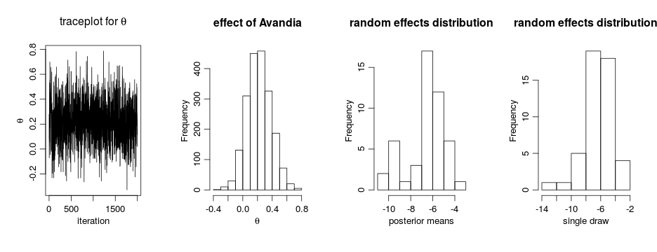
The results suggests there is an overall difference in risk between the control and treatment arms. But what about the normality assumption? Are our conclusions robust to that assumption? Perhaps the random effects distribution are skewed. (And recall that the estimates above of the random effects are generated under the normality assumption, which pushes the estimated effects to look more normal…)

DP-based random effects modeling for meta analysis

Model formulation

Now, we use a nonparametric distribution for the $\gamma_i$ s. More specifically, we assume that each $\gamma_i$ is generated from a location-scale mixture of normal distributions:

$\gamma_i \mid \mu_i, \tau_i^2 \sim \mbox{N}(\mu_i, \tau_i^2), \quad\quad (\mu_i, \tau_i^2) \mid G \sim G, \quad\quad G \sim \mbox{DP}(\alpha, H),$

where $H$ is a normal-inverse-gamma distribution.

This specification induces clustering among the random effects. As in the case of density estimation problems, the DP prior allows the data to determine the number of components, from as few as one component (i.e., simplifying to the parametric model), to as many as $n$ components, i.e., one component for each observation. This allows the distribution of the random effects to be multimodal if the data supports such behavior, greatly increasing its flexibility. This model can be specified in NIMBLE using the following code:

codeBNP <- nimbleCode({
    for(i in 1:nStudies) {
        y[i] ~ dbin(size = m[i], prob = q[i])   # avandia MIs
        x[i] ~ dbin(size = n[i], prob = p[i])   # control MIs
        q[i] <- expit(theta + gamma[i])         # Avandia log-odds
        p[i] <- expit(gamma[i])                 # control log-odds
        gamma[i] ~ dnorm(mu[i], var = tau2[i])  # random effects from mixture dist.
        mu[i] <- muTilde[xi[i]]                 # mean for random effect from cluster xi[i]
        tau2[i] <- tau2Tilde[xi[i]]             # var for random effect from cluster xi[i]
    }
    # mixture component parameters drawn from base measures
    for(i in 1:nStudies) {
        muTilde[i] ~ dnorm(mu0, var = var0)
        tau2Tilde[i] ~ dinvgamma(a0, b0)
    }
    # CRP for clustering studies to mixture components
    xi[1:nStudies] ~ dCRP(alpha, size = nStudies)
    # hyperparameters
    alpha ~ dgamma(1, 1)
    mu0 ~ dnorm(0, 10)
    var0 ~ dinvgamma(2, 1)
    a0 ~ dinvgamma(2, 1)
    b0 ~ dinvgamma(2, 1)
    theta ~ dflat()          # effect of Avandia
})

Running the MCMC

The following code compiles the model and runs a collapsed Gibbs sampler for the model

inits <- list(gamma = rnorm(nStudies), xi = sample(1:2, nStudies, replace = TRUE),
              alpha = 1, mu0 = 0, var0 = 1, a0 = 1, b0 = 1, theta = 0,
              muTilde = rnorm(nStudies), tau2Tilde = rep(1, nStudies))

samplesBNP <- nimbleMCMC(code = codeBNP, data = data, inits = inits,
               constants = constants,
               monitors = c("theta", "gamma", "alpha", "xi", "mu0", "var0", "a0", "b0"),
               thin = 10, niter = 22000, nburnin = 2000, nchains = 1, setSeed = TRUE)

## defining model...

## building model...

## setting data and initial values...

## running calculate on model (any error reports that follow may simply reflect missing values in model variables) ... 
## checking model sizes and dimensions...
## checking model calculations...
## model building finished.
## compiling... this may take a minute. Use 'showCompilerOutput = TRUE' to see C++ compiler details.
## compilation finished.
## runMCMC's handling of nburnin changed in nimble version 0.6-11. Previously, nburnin samples were discarded *post-thinning*.  Now nburnin samples are discarded *pre-thinning*.  The number of samples returned will be floor((niter-nburnin)/thin).
## running chain 1...

## |-------------|-------------|-------------|-------------|
## |-------------------------------------------------------|

gammaCols <- grep('gamma', colnames(samplesBNP))
gammaMn <- colMeans(samplesBNP[ , gammaCols])
xiCols <- grep('xi', colnames(samplesBNP))

par(mfrow = c(1,5), cex = 1.1, mgp = c(1.8,.7,0))
ts.plot(samplesBNP[ , 'theta'], xlab = 'iteration', ylab = expression(theta),
   main = expression(paste('traceplot for ', theta)))
hist(samplesBNP[ , 'theta'], xlab = expression(theta), main = 'effect of Avandia')
hist(gammaMn, xlab = 'posterior means',
              main = "random effects distrib'n")
hist(samplesBNP[1000, gammaCols], xlab = 'single draw',
                   main = "random effects distrib'n")

# How many mixture components are inferred?
xiRes <- samplesBNP[ , xiCols]
nGrps <- apply(xiRes, 1, function(x) length(unique(x)))
ts.plot(nGrps, xlab = 'iteration', ylab = 'number of components',
   main = 'number of components')

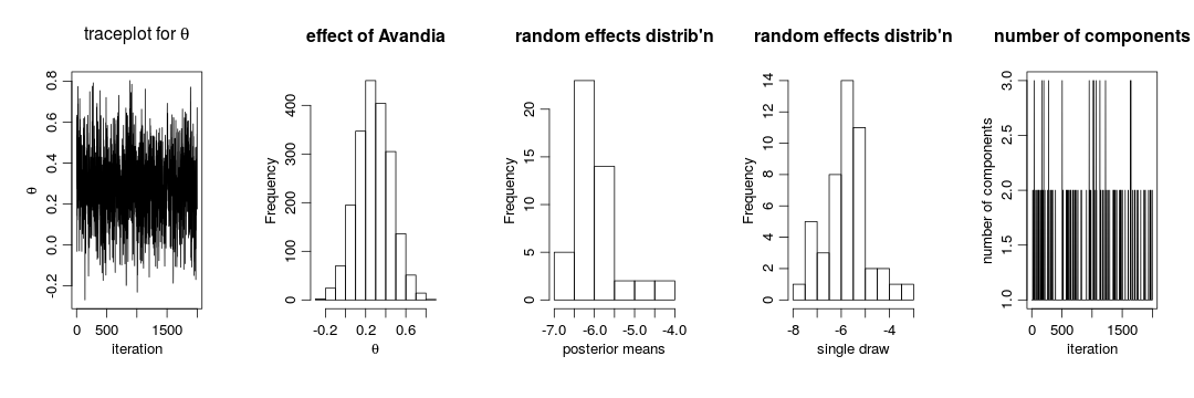
The primary inference seems robust to the original parametric assumption. This is probably driven by the fact that there is not much evidence of lack of normality in the random effects distribution (as evidenced by the fact that the posterior distribution of the number of mixture components places a large amount of probability on exactly one component).

More information and future development

Please see our User Manual for more details.

We’re in the midst of improvements to the existing BNP functionality as well as adding additional Bayesian nonparametric models, such as hierarchical Dirichlet processes and Pitman-Yor processes, so please add yourself to our announcement or user support/discussion Google groups.

Bayesian Nonparametric Models in NIMBLE, Part 1: Density Estimation

Posted on December 4, 2018December 4, 2018 by Chris Paciorek

Bayesian Nonparametric Models in NIMBLE, Part 1: Density Estimation

Bayesian nonparametrics in NIMBLE: Density estimation

Overview

In this post we illustrate NIMBLE’s BNP capabilities by showing how to use nonparametric mixture models with different kernels for density estimation. In a later post, we will take a parametric generalized linear mixed model and show how to switch to a nonparametric representation of the random effects that avoids the assumption of normally-distributed random effects.

For more detailed information on NIMBLE and Bayesian nonparametrics in NIMBLE, see the NIMBLE User Manual.

Basic density estimation using Dirichlet Process Mixture models

NIMBLE provides the machinery for nonparametric density estimation by means of Dirichlet process mixture (DPM) models (Ferguson, 1974; Lo, 1984; Escobar, 1994; Escobar and West, 1995). For an independent and identically distributed sample $y_1, \ldots, y_n$ , the model takes the form

$y_i \mid \theta_i \sim p(y_i \mid \theta_i), \quad\quad \theta_i \mid G \sim G, \quad\quad G \mid \alpha, H \sim \mbox{DP}(\alpha, H), \quad\quad i=1,\ldots, n .$

The NIMBLE implementation of this model is flexible and allows for mixtures of arbitrary kernels, $p(y_i \mid \theta)$ , which can be either conjugate or non-conjugate to the (also arbitrary) base measure $H$ . In the case of conjugate kernel / base measure pairs, NIMBLE is able to detect the presence of the conjugacy and use it to improve the performance of the sampler.

To illustrate these capabilities, we consider the estimation of the probability density function of the waiting time between eruptions of the Old Faithful volcano data set available in R.

data(faithful)

The observations $y_1, \ldots, y_n$ correspond to the second column of the dataframe, and $n = 272$ .

Fitting a location-scale mixture of Gaussian distributions using the CRP representation

Model specification

We first consider a location-scale Dirichlet process mixture of normal distributionss fitted to the transformed data $y_i^{*} = \log (y_i)$ :

$y^{*}_i \mid \mu_i, \sigma^2_i \sim \mbox{N}(\mu_i, \sigma^2_i), \quad (\mu_i, \sigma^2_i) \mid G \sim G, \quad G \mid \alpha, H \sim \mbox{DP}(\alpha, H), \quad i=1,\ldots, n,$

where $H$ corresponds to a normal-inverse-gamma distribution. This model can be interpreted as providing a Bayesian version of kernel density estimation for $y^{*}_i$ using Gaussian kernels and adaptive bandwidths. On the original scale of the data, this translates into an adaptive log-Gaussian kernel density estimate.

Introducing auxiliary variables $\xi_1, \ldots, \xi_n$ that indicate which component of the mixture generates each observation, and integrating over the random measure $G$ , we obtain the CRP representation of the model (Blackwell and MacQueen, 1973):

$y_i^{*} \mid \{ \tilde{\mu}_k \}, \{ \tilde{\sigma}_k^{2} \} \sim \mbox{N}\left( \tilde{\mu}_{\xi_i}, \tilde{\sigma}^2_{\xi_i} \right), \quad\quad \xi \mid \alpha \sim \mbox{CRP}(\alpha), \quad\quad (\tilde{\mu}_k, \tilde{\sigma}_k^2) \mid H \sim H, \quad\quad i=1,\ldots, n ,$

where

$p(\xi \mid \alpha) = \frac{\Gamma(\alpha)}{\Gamma(\alpha + n)} \alpha^{K(\xi)} \prod_k \Gamma\left(m_k(\xi)\right),$

$K(\xi) \le n$ is the number of unique values in the vector $\xi$ , and $m_k(\xi)$ is the number of times the $k$ -th unique value appears in $\xi$ . This specification makes it clear that each observation belongs to any of at most $n$ normally distributed clusters, and that the CRP distribution corresponds to the prior distribution on the partition structure.

NIMBLE’s specification of this model is given by

code <- nimbleCode({
  for(i in 1:n) {
    y[i] ~ dnorm(mu[i], var = s2[i])
    mu[i] <- muTilde[xi[i]]
    s2[i] <- s2Tilde[xi[i]]
  }
  xi[1:n] ~ dCRP(alpha, size = n)
  for(i in 1:n) {
    muTilde[i] ~ dnorm(0, var = s2Tilde[i])
    s2Tilde[i] ~ dinvgamma(2, 1)
  }
  alpha ~ dgamma(1, 1)
})

Note that in the model code the length of the parameter vectors muTilde and s2Tilde has been set to $n$ . We do this because the current implementation of NIMBLE requires that the length of vector of parameters be set in advance and does not allow for their number to change between iterations. Hence, if we are to ensure that the algorithm always performs as intended we need to work with the worst case scenario, i.e., the case where there are as many components as observations. While this ensures that the algorithm always works as intended, it is also somewhat inefficient, both in terms of memory requirements (when $n$ is large a large number of unoccupied components need to be maintained) and in terms of computational burden (a large number of parameters that are not required for posterior inference need to be updated at every iteration). When we use a mixture of gamma distributions below, we will show a computational shortcut that improves the efficiency.

Note also that the value of $\alpha$ controls the number of components we expect a priori, with larger values of $\alpha$ corresponding to a larger number of components occupied by the data. Hence, by assigning a prior to $\alpha$ we add flexibility to the model specification. The particular choice of a Gamma prior allows NIMBLE to use a data-augmentation scheme to efficiently sample from the corresponding full conditional distribution. Alternative prior specifications for $\alpha$ are possible, in which case the default sampler for this parameter is an adaptive random-walk Metropolis-Hastings algorithm.

Running the MCMC algorithm

The following code sets up the data and constants, initializes the parameters, defines the model object, and builds and runs the MCMC algorithm. Because the specification is in terms of a Chinese restaurant process, the default sampler selected by NIMBLE is a collapsed Gibbs sampler (Neal, 2000).

set.seed(1)
# Model Data
lFaithful <- log(faithful$waiting)
standlFaithful <- (lFaithful - mean(lFaithful)) / sd(lFaithful)
data <- list(y = standlFaithful)
# Model Constants
consts <- list(n = length(standlFaithful))
# Parameter initialization
inits <- list(xi = sample(1:10, size=consts$n, replace=TRUE),
              muTilde = rnorm(consts$n, 0, sd = sqrt(10)),
              s2Tilde = rinvgamma(consts$n, 2, 1),
              alpha = 1)
# Model creation and compilation
rModel <- nimbleModel(code, data = data, inits = inits, constants = consts)

## defining model...

## building model...

## setting data and initial values...

## running calculate on model (any error reports that follow may simply reflect missing values in model variables) ... 
## checking model sizes and dimensions...
## model building finished.

cModel <- compileNimble(rModel)

## compiling... this may take a minute. Use 'showCompilerOutput = TRUE' to see C++ compiler details.
## compilation finished.

# MCMC configuration, creation, and compilation
conf <- configureMCMC(rModel, monitors = c("xi", "muTilde", "s2Tilde", "alpha"))
mcmc <- buildMCMC(conf)
cmcmc <- compileNimble(mcmc, project = rModel)

## compiling... this may take a minute. Use 'showCompilerOutput = TRUE' to see C++ compiler details.
## compilation finished.

samples <- runMCMC(cmcmc, niter = 7000, nburnin = 2000, setSeed = TRUE)

## running chain 1...

## |-------------|-------------|-------------|-------------|
## |-------------------------------------------------------|

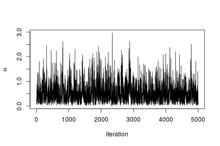
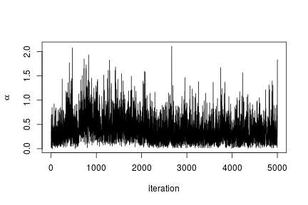
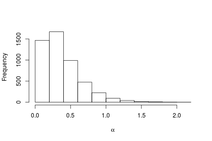
We can extract the samples from the posterior distributions of the parameters and create trace plots, histograms, and any other summary of interest. For example, for the concentration parameter $\alpha$ we have:

# Trace plot for the concentration parameter
ts.plot(samples[ , "alpha"], xlab = "iteration", ylab = expression(alpha))

# Posterior histogram
hist(samples[ , "alpha"], xlab = expression(alpha), main = "", ylab = "Frequency")

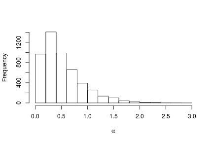
quantile(samples[ , "alpha"], c(0.5, 0.025, 0.975))

##        50%       2.5%      97.5% 
## 0.42365754 0.06021512 1.52299639

Under this model, the posterior predictive distribution for a new observation $\tilde{y}$ , $p(\tilde{y} \mid y_1, \ldots, y_n)$ , is the optimal density estimator (under squared error loss). Samples for this estimator can be easily computed from the samples generated by our MCMC:

# posterior samples of the concentration parameter
alphaSamples <- samples[ , "alpha"]
# posterior samples of the cluster means
muTildeSamples <- samples[ , grep('muTilde', colnames(samples))]
# posterior samples of the cluster variances
s2TildeSamples <- samples[ , grep('s2Tilde', colnames(samples))]
# posterior samples of the cluster memberships
xiSamples <- samples [ , grep('xi', colnames(samples))]

standlGrid <- seq(-2.5, 2.5, len = 200) # standardized grid on log scale

densitySamplesStandl <- matrix(0, ncol = length(standlGrid), nrow = nrow(samples))
for(i in 1:nrow(samples)){
  k <- unique(xiSamples[i, ])
  kNew <- max(k) + 1
  mk <- c()
  li <- 1
  for(l in 1:length(k)) {
    mk[li] <- sum(xiSamples[i, ] == k[li])
    li <- li + 1
  }
  alpha <- alphaSamples[i]

  muK <-  muTildeSamples[i, k]
  s2K <-  s2TildeSamples[i, k]
  muKnew <-  muTildeSamples[i, kNew]
  s2Knew <-  s2TildeSamples[i, kNew]

  densitySamplesStandl[i, ] <- sapply(standlGrid,
                function(x)(sum(mk * dnorm(x, muK, sqrt(s2K))) +
                alpha * dnorm(x, muKnew, sqrt(s2Knew)) )/(alpha+consts$n))
}

hist(data$y, freq = FALSE, xlim = c(-2.5, 2.5), ylim = c(0,0.75), main = "",
     xlab = "Waiting times on standardized log scale")
## pointwise estimate of the density for standardized log grid
lines(standlGrid, apply(densitySamplesStandl, 2, mean), lwd = 2, col = 'black')
lines(standlGrid, apply(densitySamplesStandl, 2, quantile, 0.025), lty = 2, col = 'black')
lines(standlGrid, apply(densitySamplesStandl, 2, quantile, 0.975), lty = 2, col = 'black')

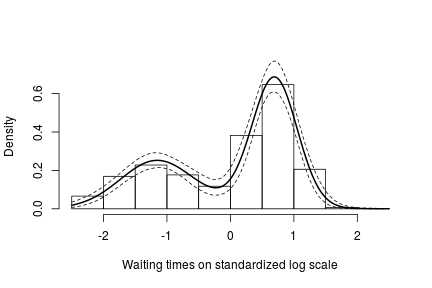
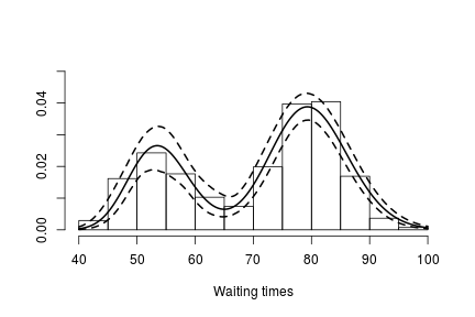
Recall, however, that this is the density estimate for the logarithm of the waiting time. To obtain the density on the original scale we need to apply the appropriate transformation to the kernel.

lgrid <- standlGrid*sd(lFaithful) + mean(lFaithful) # grid on log scale
densitySamplesl <- densitySamplesStandl / sd(lFaithful) # density samples for grid on log scale

hist(faithful$waiting, freq = FALSE, xlim = c(40, 100), ylim=c(0, 0.05),
     main = "", xlab = "Waiting times")
lines(exp(lgrid), apply(densitySamplesl, 2, mean)/exp(lgrid), lwd = 2, col = 'black')
lines(exp(lgrid), apply(densitySamplesl, 2, quantile, 0.025)/exp(lgrid), lty = 2,
      col = 'black')
lines(exp(lgrid), apply(densitySamplesl, 2, quantile, 0.975)/exp(lgrid), lty = 2,
      col = 'black')

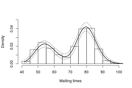
In either case, there is clear evidence that the data has two components for the waiting times.

Generating samples from the mixing distribution

While samples from the posterior distribution of linear functionals of the mixing distribution $G$ (such as the predictive distribution above) can be computed directly from the realizations of the collapsed sampler, inference for non-linear functionals of $G$ requires that we first generate samples from the mixing distribution. In NIMBLE we can get posterior samples from the random measure $G$ , using the getSamplesDPmeasure function. Note that, in order to get posterior samples from $G$ , we need to monitor all the random variables involved in its computations, i.e., the membership variable, xi, the cluster parameters, muTilde and s2Tilde, and the concentration parameter, alpha.

The following code generates posterior samples from the random measure $G$ . The cMCMC object includes the model and posterior samples from the parameters. The getSamplesDPmeasure function estimates a truncation level of $G$ , namely truncG. The posterior samples are in a matrix with $(\mbox{truncG} \cdot (p+1))$ columns, where $p$ is the dimension of the vector of parameters with distribution $G$ (in this example $p=2$ ).

outputG <- getSamplesDPmeasure(cmcmc)

## compiling... this may take a minute. Use 'showCompilerOutput = TRUE' to see C++ compiler details.

## compilation finished.

## sampleDPmeasure: Approximating the random measure by a finite stick-breaking representation with and error smaller than 1e-10, leads to a truncation level of 33.

if(packageVersion('nimble') <= '0.6-12')
  samplesG <- outputG else samplesG <- outputG$samples

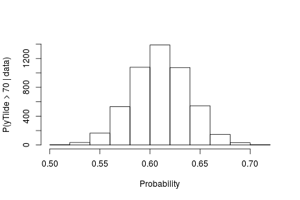
The following code computes posterior samples of $P(\tilde{y} > 70)$ using the posterior samples from the random measure $G$ . Note that these samples are computed based on the transformed model and a value larger than 70 corresponds to a value larger than 0.03557236 on the above defined grid.

if(packageVersion('nimble') >= '0.6.13')
     truncG <- outputG$trunc # truncation level for G

weightIndex <- grep('weight', colnames(samplesG))
muTildeIndex <- grep('muTilde', colnames(samplesG))
s2TildeIndex <- grep('s2Tilde', colnames(samplesG))

probY70 <- rep(0, nrow(samples))  # posterior samples of P(y.tilde > 70)
for(i in seq_len(nrow(samples))) {
  probY70[i] <- sum(samplesG[i, weightIndex] *
                    pnorm(0.03557236, mean = samplesG[i, muTildeIndex],
                      sd = sqrt(samplesG[i, s2TildeIndex]), lower.tail = FALSE))
}

hist(probY70,  xlab = "Probability", ylab = "P(yTilde > 70 | data)" , main = "" )

Fitting a mixture of gamma distributions using the CRP representation

NIMBLE is not restricted to using Gaussian kernels in DPM models. In the case of the Old Faithful data, an alternative to the mixture of Gaussian kernels on the logarithmic scale that we presented in the previous section is a (scale-and-shape) mixture of Gamma distributions on the original scale of the data.

Model specification

In this case, the model takes the form

$y_i \mid \{ \tilde{\beta}_k \}, \{ \tilde{\lambda}_k \} \sim \mbox{Gamma}\left( \tilde{\beta}_{\xi_i}, \tilde{\lambda}_{\xi_i} \right), \quad\quad \xi \mid \alpha \sim \mbox{CRP}(\alpha), \quad\quad (\tilde{\beta}_k, \tilde{\lambda}_k) \mid H \sim H ,$

where $H$ corresponds to the product of two independent Gamma distributions. The following code provides the NIMBLE specification for the model:

code <- nimbleCode({
  for(i in 1:n) {
    y[i] ~ dgamma(shape = beta[i], scale = lambda[i])
    beta[i] <- betaTilde[xi[i]]
    lambda[i] <- lambdaTilde[xi[i]]
  }
  xi[1:n] ~ dCRP(alpha, size = n)
  for(i in 1:50) { # only 50 cluster parameters
    betaTilde[i] ~ dgamma(shape = 71, scale = 2)
    lambdaTilde[i] ~ dgamma(shape = 2, scale = 2)
  }
  alpha ~ dgamma(1, 1)
})

Note that in this case the vectors betaTilde and lambdaTilde have length $50 \ll n = 272$ . This is done to reduce the computational and storage burdens associated with the sampling algorithm. You could think about this approach as truncating the process, except that it can be thought of as an *exact* truncation. Indeed, under the CRP representation, using parameter vector(s) with a length that is shorter than the number of observations in the sample will lead to a proper algorithm as long as the number of components instatiated by the sampler is strictly lower than the length of the parameter vector(s) for every iteration of the sampler.

Running the MCMC algorithm

The following code sets up the model data and constants, initializes the parameters, defines the model object, and builds and runs the MCMC algorithm for the mixture of Gamma distributions. Note that, when building the MCMC, a warning message about the number of cluster parameters is generated. This is because the lengths of betaTilde and lambdaTilde are smaller than $n$ . Also, note that no error message is generated during execution, which indicates that the number of clusters required never exceeded the maximum of 50.

data <- list(y = faithful$waiting)
set.seed(1)
inits <- list(xi = sample(1:10, size=consts$n, replace=TRUE),
              betaTilde = rgamma(50, shape = 71, scale = 2),
              lambdaTilde = rgamma(50, shape = 2, scale = 2),
              alpha = 1)
rModel <- nimbleModel(code, data = data, inits = inits, constants = consts)

## defining model...

## building model...

## setting data and initial values...

## running calculate on model (any error reports that follow may simply reflect missing values in model variables) ... 
## checking model sizes and dimensions...
## model building finished.

cModel <- compileNimble(rModel)

## compiling... this may take a minute. Use 'showCompilerOutput = TRUE' to see C++ compiler details.
## compilation finished.

conf <- configureMCMC(rModel, monitors = c("xi", "betaTilde", "lambdaTilde", "alpha"))
mcmc <- buildMCMC(conf)

## Warning in samplerFunction(model = model, mvSaved = mvSaved, target = target, : sampler_CRP: The number of cluster parameters is less than the number of potential clusters. The MCMC is not strictly valid if ever it proposes more components than cluster parameters exist; NIMBLE will warn you if this occurs.

cmcmc <- compileNimble(mcmc, project = rModel)

## compiling... this may take a minute. Use 'showCompilerOutput = TRUE' to see C++ compiler details.
## compilation finished.

samples <- runMCMC(cmcmc, niter = 7000, nburnin = 2000, setSeed = TRUE)

## running chain 1...

## |-------------|-------------|-------------|-------------|
## |-------------------------------------------------------|

In this case we use the posterior samples of the parameters to construct a trace plot and estimate the posterior distribution of $\alpha$ :

# Trace plot of the posterior samples of the concentration parameter
ts.plot(samples[ , 'alpha'], xlab = "iteration", ylab = expression(alpha))

# Histogram of the posterior samples for the concentration parameter 
hist(samples[ , 'alpha'], xlab = expression(alpha), ylab = "Frequency", main = "")

Generating samples from the mixing distribution

As before, we obtain samples from the posterior distribution of $G$ using the getSamplesDPmeasure function.

outputG <- getSamplesDPmeasure(cmcmc)

## compiling... this may take a minute. Use 'showCompilerOutput = TRUE' to see C++ compiler details.

## compilation finished.

## sampleDPmeasure: Approximating the random measure by a finite stick-breaking representation with and error smaller than 1e-10, leads to a truncation level of 28.

if(packageVersion('nimble') <= '0.6-12')
  samplesG <- outputG else samplesG <- outputG$samples

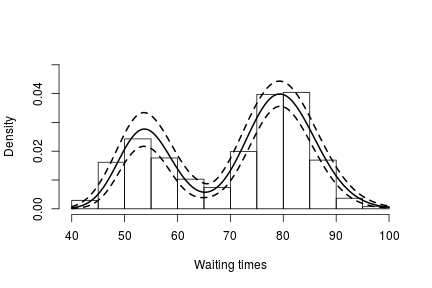
We use these samples to create an estimate of the density of the data along with a pointwise 95% credible band:

if(packageVersion('nimble') >= '0.6.13')
     truncG <- outputG$trunc # truncation level for G
grid <- seq(40, 100, len = 200)

weightSamples <- samplesG[ , grep('weight', colnames(samplesG))]
betaTildeSamples <- samplesG[ , grep('betaTilde', colnames(samplesG))]
lambdaTildeSamples <- samplesG[ , grep('lambdaTilde', colnames(samplesG))]

densitySamples <- matrix(0, ncol = length(grid), nrow = nrow(samples))
for(iter in seq_len(nrow(samples))) {
  densitySamples[iter, ] <- sapply(grid, function(x)
    sum( weightSamples[iter, ] * dgamma(x, shape = betaTildeSamples[iter, ],
                scale = lambdaTildeSamples[iter, ])))
}


hist(faithful$waiting, freq = FALSE, xlim = c(40,100), ylim = c(0, .05), main = "",
   ylab = "", xlab = "Waiting times")
lines(grid, apply(densitySamples, 2, mean), lwd = 2, col = 'black')
lines(grid, apply(densitySamples, 2, quantile, 0.025), lwd = 2, lty = 2, col = 'black')
lines(grid, apply(densitySamples, 2, quantile, 0.975), lwd = 2, lty = 2, col = 'black')

Again, we see that the density of the data is bimodal, and looks very similar to the one we obtained before.

Fitting a DP mixture of Gammas using a stick-breaking representation

Model specification

An alternative representation of the Dirichlet process mixture uses the stick-breaking representation of the random distribution $G$ (Sethuraman, 1994). NIMBLE allows us to specify an approximation that involves a truncation of the Dirichlet process to a finite number of atoms, $L$ . The resulting model therefore reduces to a finite mixture with $L$ components and a very particular prior on the weights of the mixture components.

Introducing auxiliary variables, $z_1, \ldots, z_n$ , that indicate which component generated each observation, the corresponding model for the mixture of Gamma densities discussed in the previous section takes the form

$y_i \mid \{ {\beta}_k^{\star} \}, \{ {\lambda}_k^{\star} \}, z_i \sim \mbox{Gamma}\left( {\beta}_{z_i}^{\star}, {\lambda}_{z_i}^{\star} \right), \quad\quad \boldsymbol{z} \mid \boldsymbol{w} \sim \mbox{Discrete}(\boldsymbol{w}), \quad\quad ({\beta}_k^{\star}, {\lambda}_k^{\star}) \mid H \sim H ,$

where $H$ is again the product of two independent Gamma distributions,

$w_1=v_1, \quad\quad w_l=v_l\prod_{m=1}^{l-1}(1-v_m), \quad l=2, \ldots, L-1,\quad\quad w_L=\prod_{m=1}^{L-1}(1-v_m)$

with $v_l \mid \alpha\sim \mbox{Beta}(1, \alpha), l=1, \ldots, L-1$ . The following code provides the NIMBLE specification for the model:

code <- nimbleCode(
  {
    for(i in 1:n) {
      y[i] ~ dgamma(shape = beta[i], scale = lambda[i])
      beta[i] <- betaStar[z[i]]
      lambda[i] <- lambdaStar[z[i]]
      z[i] ~ dcat(w[1:Trunc])
    }
    for(i in 1:(Trunc-1)) { # stick-breaking variables
      v[i] ~ dbeta(1, alpha)
    }
    w[1:Trunc] <- stick_breaking(v[1:(Trunc-1)]) # stick-breaking weights
    for(i in 1:Trunc) {
      betaStar[i] ~ dgamma(shape = 71, scale = 2)
      lambdaStar[i] ~ dgamma(shape = 2, scale = 2)
    }
    alpha ~ dgamma(1, 1)
  }
)

Note that the truncation level $L$ of $G$ has been set to a value Trunc, which is to be defined in the constants argument of the nimbleModel function.

Running the MCMC algorithm

data <- list(y = faithful$waiting)
set.seed(1)
consts <- list(n = length(faithful$waiting), Trunc = 50)
inits <- list(betaStar = rgamma(consts$Trunc, shape = 71, scale = 2),
              lambdaStar = rgamma(consts$Trunc, shape = 2, scale = 2),
              v = rbeta(consts$Trunc-1, 1, 1),
              z = sample(1:10, size = consts$n, replace = TRUE),
              alpha = 1)

rModel <- nimbleModel(code, data = data, inits = inits, constants = consts)

## defining model...

## building model...

## setting data and initial values...

## running calculate on model (any error reports that follow may simply reflect missing values in model variables) ... 
## checking model sizes and dimensions...
## model building finished.

cModel <- compileNimble(rModel)

## compiling... this may take a minute. Use 'showCompilerOutput = TRUE' to see C++ compiler details.
## compilation finished.

conf <- configureMCMC(rModel, monitors = c("w", "betaStar", "lambdaStar", 'z', 'alpha'))
mcmc <- buildMCMC(conf)
cmcmc <- compileNimble(mcmc, project = rModel)

## compiling... this may take a minute. Use 'showCompilerOutput = TRUE' to see C++ compiler details.
## compilation finished.

samples <- runMCMC(cmcmc, niter = 24000, nburnin = 4000, setSeed = TRUE)

## running chain 1...

## |-------------|-------------|-------------|-------------|
## |-------------------------------------------------------|

Using the stick-breaking approximation automatically provides an approximation, $G_L$ , of the random distribution $G$ . The following code computes posterior samples of $G_L$ using posterior samples from the samples object, and from them, a density estimate for the data.

betaStarSamples <- samples[ , grep('betaStar', colnames(samples))]
lambdaStarSamples <- samples[ , grep('lambdaStar', colnames(samples))]
weightSamples <- samples[ , grep('w', colnames(samples))]

grid <- seq(40, 100, len = 200)

densitySamples <- matrix(0, ncol = length(grid), nrow = nrow(samples))
for(i in 1:nrow(samples)) {
  densitySamples[i, ] <- sapply(grid, function(x)
    sum(weightSamples[i, ] * dgamma(x, shape = betaStarSamples[i, ],
                                    scale = lambdaStarSamples[i, ])))
}

hist(faithful$waiting, freq = FALSE,  xlab = "Waiting times", ylim=c(0,0.05),
     main = '')
lines(grid, apply(densitySamples, 2, mean), lwd = 2, col = 'black')
lines(grid, apply(densitySamples, 2, quantile, 0.025), lwd = 2, lty = 2, col = 'black')
lines(grid, apply(densitySamples, 2, quantile, 0.975), lwd = 2, lty = 2, col = 'black')

As expected, this estimate looks identical to the one we obtained through the CRP representation of the process.

More information and future development

Please see our User Manual for more details.

References

Blackwell, D. and MacQueen, J. 1973. Ferguson distributions via Polya urn schemes. The Annals of Statistics 1:353-355.

Ferguson, T.S. 1974. Prior distribution on the spaces of probability measures. Annals of Statistics 2:615-629.

Lo, A.Y. 1984. On a class of Bayesian nonparametric estimates I: Density estimates. The Annals of Statistics 12:351-357.

Escobar, M.D. 1994. Estimating normal means with a Dirichlet process prior. Journal of the American Statistical Association 89:268-277.

Escobar, M.D. and West, M. 1995. Bayesian density estimation and inference using mixtures. Journal of the American Statistical Association 90:577-588.

Ishwaran, H. and James, L.F. 2001. Gibbs sampling methods for stick-breaking priors. Journal of the American Statistical Association 96: 161-173.

Ishwaran, H. and James, L.F. 2002. Approximate Dirichlet process computing in finite normal mixtures: smoothing and prior information. Journal of Computational and Graphical Statistics 11:508-532.

Neal, R. 2000. Markov chain sampling methods for Dirichlet process mixture models. Journal of Computational and Graphical Statistics 9:249-265.

Sethuraman, J. 1994. A constructive definition of Dirichlet prior. Statistica Sinica 2: 639-650.

Spread the word: NIMBLE is looking for a post-doc

Posted on September 13, 2018September 13, 2018 by nimble-admin

We have an opening for a post-doctoral scholar to work on methods for and applications of hierarchical statistical models using the NIMBLE software (https://r-nimble.org) at the University of California, Berkeley. NIMBLE is an R package that combines a new implementation of a model language similar to BUGS/JAGS, a system for writing new algorithms and MCMC samplers, and a compiler that generates C++ for each model and set of algorithms. The successful candidate will work with Chris Paciorek, Perry de Valpine, and potentially other NIMBLE collaborators to pursue a research program with a combination of building and applying methods in NIMBLE. Specific methods and application areas will be determined based on interests of the successful candidate. Applicants should have a Ph.D. in Statistics or a related discipline. We are open to non-Ph.D. candidates who can make a compelling case that they have relevant experience. The position is funded for two years, with an expected start date between October 2018 and June 2019. Applicants should send a cover letter, including a statement of how their interests relate to NIMBLE, the names of three references, and a CV to nimble.stats@gmail.com, with “NIMBLE post-doc application” in the subject. Applications will be considered on a rolling basis starting 15 October, 2018.

Version 0.6-12 of NIMBLE released

Posted on July 29, 2018July 29, 2018 by Chris Paciorek

We’ve released the newest version of NIMBLE on CRAN and on our website. Version 0.6-12 is primarily a maintenance release with various bug fixes.

Changes include:

a fix for the bootstrap particle filter to correctly calculate weights when particles are not resampled (the filter had been omitting the previous weights when calculating the new weights);
addition of an option to print MCMC samplers of a particular type;
avoiding an overly-aggressive check for ragged arrays when building models; and
avoiding assigning a sampler to non-conjugacy inverse-Wishart nodes (thereby matching our handling of Wishart nodes).

Please see the NEWS file in the installed package for more details.

Version 0.6-11 of NIMBLE released

Posted on June 16, 2018June 16, 2018 by Chris Paciorek

We’ve released the newest version of NIMBLE on CRAN and on our website.

Version 0.6-11 has important new features, notably support for Bayesian nonparametric mixture modeling, and more are on the way in the next few months.

New features include:

support for Bayesian nonparametric mixture modeling using Dirichlet process mixtures, with specialized MCMC samplers automatically assigned in NIMBLE’s default MCMC (See Chapter 10 of the manual for details);
additional resampling methods available with the auxiliary and bootstrap particle filters;
user-defined filtering algorithms can be used with NIMBLE’s particle MCMC samplers;
MCMC thinning intervals can be modified at MCMC run-time;
both runMCMC() and nimbleMCMC() now drop burn-in samples before thinning, making their behavior consistent with each other;
increased functionality for the ‘setSeed’ argument in nimbleMCMC() and runMCMC();
new functionality for specifying the order in which sampler functions are executed in an MCMC; and
invalid dynamic indexes now result in a warning and NaN values but do not cause execution to error out, allowing MCMC sampling to continue.

Please see the NEWS file in the installed package for more details

Quick guide for converting from JAGS or BUGS to NIMBLE

Posted on May 30, 2018May 30, 2018 by nimble-admin

Converting to NIMBLE from JAGS, OpenBUGS or WinBUGS

NIMBLE is a hierarchical modeling package that uses nearly the same modeling language as the popular MCMC packages WinBUGS, OpenBUGS and JAGS. NIMBLE makes the modeling language extensible — you can add distributions and functions — and also allows customization of MCMC or other algorithms that use models. Here is a quick summary of steps to convert existing code from WinBUGS, OpenBUGS or JAGS to NIMBLE. For more information, see examples on r-nimble.org or the NIMBLE User Manual.

Main steps for converting existing code

These steps assume you are familiar with running WinBUGS, OpenBUGS or JAGS through an R package such as R2WinBUGS, R2jags, rjags, or jagsUI.

Wrap your model code in nimbleCode({}), directly in R.

This replaces the step of writing or generating a separate file containing the model code.
Alternatively, you can read standard JAGS- and BUGS-formatted code and data files using
readBUGSmodel.

Provide information about missing or empty indices

Example: If x is a matrix, you must write at least x[,] to show it has two dimensions.
If other declarations make the size of x clear, x[,] will work in some circumstances.
If not, either provide index ranges (e.g. x[1:n, 1:m]) or use the dimensions argument to nimbleModel to provide the sizes in each dimension.

Choose how you want to run MCMC.

Use nimbleMCMC() as the just-do-it way to run an MCMC. This will take all steps to
set up and run an MCMC using NIMBLE’s default configuration.
To use NIMBLE’s full flexibility: build the model, configure and build the MCMC, and compile both the model and MCMC. Then run the MCMC via runMCMC or by calling the run function of the compiled MCMC. See the NIMBLE User Manual to learn more about what you can do.

See below for a list of some more nitty-gritty additional steps you may need to consider for some models.

Example: An animal abundance model

This example is adapted from Chapter 6, Section 6.4 of Applied Hierarchical Modeling in Ecology: Analysis of distribution, abundance and species richness in R and BUGS. Volume I: Prelude and Static Models by Marc Kéry and J. Andrew Royle (2015, Academic Press). The book’s web site provides code for its examples.

Original code

The original model code looks like this:


cat(file = "model2.txt","
model {
# Priors
for(k in 1:3){                # Loop over 3 levels of hab or time factors
   alpha0[k] ~ dunif(-10, 10) # Detection intercepts
   alpha1[k] ~ dunif(-10, 10) # Detection slopes
   beta0[k] ~ dunif(-10, 10)  # Abundance intercepts
   beta1[k] ~ dunif(-10, 10)  # Abundance slopes
}

# Likelihood
# Ecological model for true abundance
for (i in 1:M){
   N[i] ~ dpois(lambda[i])
   log(lambda[i]) <- beta0[hab[i]] + beta1[hab[i]] * vegHt[i]
   # Some intermediate derived quantities
   critical[i] <- step(2-N[i])# yields 1 whenever N is 2 or less
   z[i] <- step(N[i]-0.5)     # Indicator for occupied site
   # Observation model for replicated counts
   for (j in 1:J){
      C[i,j] ~ dbin(p[i,j], N[i])
      logit(p[i,j]) <- alpha0[j] + alpha1[j] * wind[i,j]
   }
}

# Derived quantities
Nocc <- sum(z[])         # Number of occupied sites among sample of M
Ntotal <- sum(N[])       # Total population size at M sites combined
Nhab[1] <- sum(N[1:33])  # Total abundance for sites in hab A
Nhab[2] <- sum(N[34:66]) # Total abundance for sites in hab B
Nhab[3] <- sum(N[67:100])# Total abundance for sites in hab C
for(k in 1:100){         # Predictions of lambda and p ...
   for(level in 1:3){    #    ... for each level of hab and time factors
      lam.pred[k, level] <- exp(beta0[level] + beta1[level] * XvegHt[k])
      logit(p.pred[k, level]) <- alpha0[level] + alpha1[level] * Xwind[k]
   }
}
N.critical <- sum(critical[]) # Number of populations with critical size
}")

Brief summary of the model

This is known as an "N-mixture" model in ecology. The details aren't really important for illustrating the mechanics of converting this model to NIMBLE, but here is a brief summary anyway. The latent abundances N[i] at sites i = 1...M are assumed to follow a Poisson. The j-th count at the i-th site, C[i, j], is assumed to follow a binomial with detection probability p[i, j]. The abundance at each site depends on a habitat-specific intercept and coefficient for vegetation height, with a log link. The detection probability for each sampling occasion depends on a date-specific intercept and coefficient for wind speed. Kéry and Royle concocted this as a simulated example to illustrate the hierarchical modeling approaches for estimating abundance from count data on repeated visits to multiple sites.

NIMBLE version of the model code

Here is the model converted for use in NIMBLE. In this case, the only changes to the code are to insert some missing index ranges (see comments).

library(nimble)
Section6p4_code <- nimbleCode( {
    # Priors
    for(k in 1:3) {                # Loop over 3 levels of hab or time factors
      alpha0[k] ~ dunif(-10, 10) # Detection intercepts
      alpha1[k] ~ dunif(-10, 10) # Detection slopes
      beta0[k] ~ dunif(-10, 10)  # Abundance intercepts
      beta1[k] ~ dunif(-10, 10)  # Abundance slopes
    }

    # Likelihood
    # Ecological model for true abundance
    for (i in 1:M){
      N[i] ~ dpois(lambda[i])
      log(lambda[i]) <- beta0[hab[i]] + beta1[hab[i]] * vegHt[i]
      # Some intermediate derived quantities
      critical[i] <- step(2-N[i])# yields 1 whenever N is 2 or less
      z[i] <- step(N[i]-0.5)     # Indicator for occupied site
      # Observation model for replicated counts
      for (j in 1:J){
        C[i,j] ~ dbin(p[i,j], N[i])
        logit(p[i,j]) <- alpha0[j] + alpha1[j] * wind[i,j]
        }
    }

    # Derived quantities; unnececssary when running for inference purpose
    # NIMBLE: We have filled in indices in the next two lines.
    Nocc <- sum(z[1:100])         # Number of occupied sites among sample of M
    Ntotal <- sum(N[1:100])       # Total population size at M sites combined
    Nhab[1] <- sum(N[1:33])  # Total abundance for sites in hab A
    Nhab[2] <- sum(N[34:66]) # Total abundance for sites in hab B
    Nhab[3] <- sum(N[67:100])# Total abundance for sites in hab C
    for(k in 1:100){         # Predictions of lambda and p ...
      for(level in 1:3){    #    ... for each level of hab and time factors
        lam.pred[k, level] <- exp(beta0[level] + beta1[level] * XvegHt[k])
        logit(p.pred[k, level]) <- alpha0[level] + alpha1[level] * Xwind[k]
        }
      }
    # NIMBLE: We have filled in indices in the next line. 
    N.critical <- sum(critical[1:100]) # Number of populations with critical size
  })

Simulated data

To carry this example further, we need some simulated data. Kéry and Royle provide separate code to do this. With NIMBLE we could use the model itself to simulate data rather than writing separate simulation code. But for our goals here, we simply copy Kéry and Royle's simulation code, and we compact it somewhat:

# Code from Kery and Royle (2015)
# Choose sample sizes and prepare obs. data array y
set.seed(1)                   # So we all get same data set
M <- 100                      # Number of sites
J <- 3                        # Number of repeated abundance measurements
C <- matrix(NA, nrow = M, ncol = J) # to contain the observed data

# Create a covariate called vegHt
vegHt <- sort(runif(M, -1, 1)) # sort for graphical convenience

# Choose parameter values for abundance model and compute lambda
beta0 <- 0                    # Log-scale intercept
beta1 <- 2                    # Log-scale slope for vegHt
lambda <- exp(beta0 + beta1 * vegHt) # Expected abundance

# Draw local abundance
N <- rpois(M, lambda)

# Create a covariate called wind
wind <- array(runif(M * J, -1, 1), dim = c(M, J))

# Choose parameter values for measurement error model and compute detectability
alpha0 <- -2                        # Logit-scale intercept
alpha1 <- -3                        # Logit-scale slope for wind
p <- plogis(alpha0 + alpha1 * wind) # Detection probability

# Take J = 3 abundance measurements at each site
for(j in 1:J) {
  C[,j] <- rbinom(M, N, p[,j])
}

# Create factors
time <- matrix(rep(as.character(1:J), M), ncol = J, byrow = TRUE)
hab <- c(rep("A", 33), rep("B", 33), rep("C", 34))  # assumes M = 100

# Bundle data
# NIMBLE: For full flexibility, we could separate this list
#         into constants and data lists.  For simplicity we will keep
#         it as one list to be provided as the "constants" argument.
#         See comments about how we would split it if desired.
win.data <- list(
    ## NIMBLE: C is the actual data
    C = C,
    ## NIMBLE: Covariates can be data or constants
    ##         If they are data, you could modify them after the model is built
    wind = wind,
    vegHt = vegHt,
    XvegHt = seq(-1, 1,, 100), # Used only for derived quantities
    Xwind = seq(-1, 1,,100),   # Used only for derived quantities
    ## NIMBLE: The rest of these are constants, needed for model definition
    ## We can provide them in the same list and NIMBLE will figure it out.
    M = nrow(C),
    J = ncol(C),
    hab = as.numeric(factor(hab))
)

Initial values

Next we need to set up initial values and choose parameters to monitor in the MCMC output. To do so we will again directly use Kéry and Royle's code.

Nst <- apply(C, 1, max)+1   # Important to give good inits for latent N
inits <- function() list(N = Nst,
                         alpha0 = rnorm(3),
                         alpha1 = rnorm(3),
                         beta0 = rnorm(3),
                         beta1 = rnorm(3))

# Parameters monitored
# could also estimate N, bayesian counterpart to BUPs before: simply add "N" to the list
params <- c("alpha0", "alpha1", "beta0", "beta1", "Nocc", "Ntotal", "Nhab", "N.critical", "lam.pred", "p.pred")

Run MCMC with `nimbleMCMC`

Now we are ready to run an MCMC in nimble. We will run only one chain, using the same settings as Kéry and Royle.

samples <- nimbleMCMC(
    code = Section6p4_code,
    constants = win.data, ## provide the combined data & constants as constants
    inits = inits,
    monitors = params,
    niter = 22000,
    nburnin = 2000,
    thin = 10)

## defining model...

## Detected C as data within 'constants'.

## Adding C as data for building model.

## building model...

## setting data and initial values...

## running calculate on model (any error reports that follow may simply reflect missing values in model variables) ... 
## checking model sizes and dimensions...
## checking model calculations...
## model building finished.
## compiling... this may take a minute. Use 'showCompilerOutput = TRUE' to see C++ compiler details.
## compilation finished.
## runMCMC's handling of nburnin changed in nimble version 0.6-11. Previously, nburnin samples were discarded *post-thinning*.  Now nburnin samples are discarded *pre-thinning*.  The number of samples returned will be floor((niter-nburnin)/thin).
## running chain 1...

## |-------------|-------------|-------------|-------------|
## |-------------------------------------------------------|

Work with the samples

Finally we want to look at our samples. NIMBLE returns samples as a simple matrix with named columns. There are numerous packages for processing MCMC output. If you want to use the coda package, you can convert a matrix to a coda mcmc object like this:

library(coda)
coda.samples <- as.mcmc(samples)

Alternatively, if you call nimbleMCMC with the argument samplesAsCodaMCMC = TRUE, the samples will be returned as a coda object.

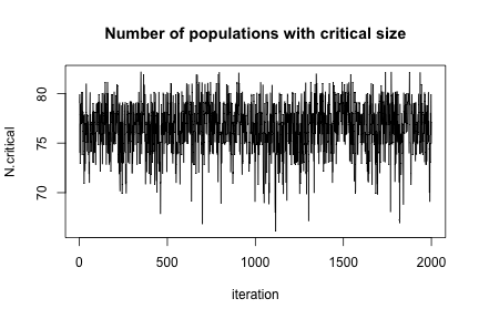
To show that MCMC really happened, here is a plot of N.critical:

plot(jitter(samples[, "N.critical"]), xlab = "iteration", ylab = "N.critical",
     main = "Number of populations with critical size",
     type = "l")

Next steps

NIMBLE allows users to customize MCMC and other algorithms in many ways. See the NIMBLE User Manual and web site for more ideas.

Smaller steps you may need for converting existing code

If the main steps above aren't sufficient, consider these additional steps when converting from JAGS, WinBUGS or OpenBUGS to NIMBLE.

Convert any use of truncation syntax
- e.g. x ~ dnorm(0, tau) T(a, b) should be re-written as x ~ T(dnorm(0, tau), a, b).
- If reading model code from a file using readBUGSmodel, the x ~ dnorm(0, tau) T(a, b) syntax will work.
Possibly split the data into data and constants for NIMBLE.
- NIMBLE has a more general concept of data, so NIMBLE makes a distinction between data and constants.
- Constants are necessary to define the model, such as nsite in for(i in 1:nsite) {...} and constant vectors of factor indices (e.g. block in mu[block[i]]).
- Data are observed values of some variables.
- Alternatively, one can provide a list of both constants and data for the constants argument to nimbleModel, and NIMBLE will try to determine which is which. Usually this will work, but when in doubt, try separating them.
Possibly update initial values (inits).
- In some cases, NIMBLE likes to have more complete inits than the other packages.
- In a model with stochastic indices, those indices should have inits values.
- When using nimbleMCMC or runMCMC, inits can be a function, as in R packages for calling WinBUGS, OpenBUGS or JAGS. Alternatively, it can be a list.
- When you build a model with nimbleModel for more control than nimbleMCMC, you can provide inits as a list. This sets defaults that can be over-ridden with the inits argument to runMCMC.

Two day workshop: Flexible programming of MCMC and other methods for hierarchical and Bayesian models

Posted on April 19, 2018April 19, 2018 by Chris Paciorek

We’ll be giving a two day workshop at the 43rd Annual Summer Institute of Applied Statistics at Brigham Young University (BYU) in Utah, June 19-20, 2018.

Abstract is below, and registration and logistics information can be found here.

This workshop provides a hands-on introduction to using, programming, and sharing Bayesian and hierarchical modeling algorithms using NIMBLE (r-nimble.org). In addition to learning the NIMBLE system, users will develop hands-on experience with various computational methods. NIMBLE is an R-based system that allows one to fit models specified using BUGS/JAGS syntax but with much more flexibility in defining the statistical model and the algorithm to be used on the model. Users operate from within R, but NIMBLE generates C++ code for models and algorithms for fast computation. I will open with an overview of creating a hierarchical model and fitting the model using a basic MCMC, similarly to how one can use WinBUGS, JAGS, and Stan. I will then discuss how NIMBLE allows the user to modify the MCMC – changing samplers and specifying blocking of parameters. Next I will show how to extend the BUGS syntax with user-defined distributions and functions that provide flexibility in specifying a statistical model of interest. With this background we can then explore the NIMBLE programming system, which allows one to write new algorithms not already provided by NIMBLE, including new MCMC samplers, using a subset of the R language. I will then provide examples of non-MCMC algorithms that have been programmed in NIMBLE and how algorithms can be combined together, using the example of a particle filter embedded within an MCMC. We will see new functionality in NIMBLE that allows one to fit Bayesian nonparametric models and spatial models. I will close with a discussion of how NIMBLE enables sharing of new methods and reproducibility of research. The workshop will include a number of breakout periods for participants to use and program MCMC and other methods, either on example problems or problems provided by participants. In addition, participants will see NIMBLE’s flexibility in action in several real problems.

Bayesian nonparametrics in NIMBLE: Nonparametric random effects

Overview

Parametric meta analysis of Avandia myocardial infarctions (MIs)

Model formulation

Running the MCMC

DP-based random effects modeling for meta analysis

Model formulation

Running the MCMC

More information and future development

Bayesian nonparametrics in NIMBLE: Density estimation

Overview

Basic density estimation using Dirichlet Process Mixture models

Fitting a location-scale mixture of Gaussian distributions using the CRP representation

Model specification

Running the MCMC algorithm

Generating samples from the mixing distribution

Fitting a mixture of gamma distributions using the CRP representation

Model specification

Running the MCMC algorithm

Generating samples from the mixing distribution

Fitting a DP mixture of Gammas using a stick-breaking representation

Model specification

Running the MCMC algorithm

More information and future development

References

Converting to NIMBLE from JAGS, OpenBUGS or WinBUGS

Main steps for converting existing code

Example: An animal abundance model

Original code

Brief summary of the model

NIMBLE version of the model code

Simulated data

Initial values

Run MCMC with nimbleMCMC

Work with the samples

Next steps

Smaller steps you may need for converting existing code

Leave a Reply Cancel reply

Run MCMC with `nimbleMCMC`